Instructor Notes
This is a placeholder file. Please add content here.
Introduction
Instructor Note
Given that this curriculum deals explicitly with Indigenous data sovereignty and governance, it is advisable to start with a land acknowledgement.
For Albuquerque, NM (the location of the first offering of this curriculum) here is info UNM’s land acknowledgement and the process leading up to it: - https://diverse.unm.edu/about-dei-at-unm/land-labor-acknowledgement.html - https://diverse.unm.edu/assets/documents/unm-indigenous-peoples-land-and-territory-acknowledgment-brown-paper.pdf
Any land acknowledgement should be done in the context of growing awareness that the intentions of many land acknowledgements, while aspiring to be good intentions, where ill-informed and the acknowledgements have led to harm in some cases. Here are resources to read about that: - https://nativegov.org/news/beyond-land-acknowledgment-guide/ - https://hyperallergic.com/769024/your-land-acknowledgment-is-not-enough/ - https://www.pbs.org/newshour/nation/analysis-how-well-meaning-land-acknowledgements-can-erase-indigenous-people-and-sanitize-history
It is becoming agreed upon protocol that land acknowledgements should be given only in the context of how the event or institution presenting the land acknowledgement engages with activities beyond an otherwise hollow “acknowledgement” of unceded lands.
Instructor Note
A note on Native Land Digital map: the map loads with a disclaimer that is important to read: the geospatial polygons are not necessarily approved by the groups they purport to represent. Native Land Digital is Native-led and has a mechanism to verify polygons, but there might be more accurate map representations you can use for your areas.
A note on relational intros: if giving this curriculum live you could choose to demonstrate yourselves (as instructors) the different types of introductions modeled by Dr. Kat Gardner-Vandy and Daniella Scalice, or you could show the video. Note that it’s a legit consideration about the length of the relational introduction to allow time and space for everybody to get through their introductions; more people = more succinct intros.
Instructor Note
Transition to data narrative.
Instructor Note
Instead of “…the Indigenous land where we gather…” you could reference the specific communities.
Instructor Note
Slide deck in /instructors/hawaii_4_dim_data.pdf
Instructor Note
Breakout groups or collaborate on the white board.
Indigenous Data Sovereignty and the CARE Principles
Instructor Note
Give the slide show; slide deck is /instructors/local_contexts-care.pdf
Instructor Note
Give a tour of your own Local Contexts Hub account
Abundance DataIntroduction to abundance dataWorking with abundance dataRecap
Instructor Note
Sometimes gnr_resolve doesnt work. From the
taxize documentation:
503 Service Unavailable: This is typically a temporary problem; often given when a server is handling too many requests, and is briefly down.
Instructor Note
Go to google and you’ll see that Agrotis chersotoides is a synonym of Peridroma chersotoides, while Metrothorax deverilli is a valid species with little information about it, thus it doesn’t show up in GNR.
Trait dataHill numbers
Summarizing phylogenetic data
Instructor Note
Learners should have the object abundances already in
their environment, from the previous episode. If not, use line
below.
R
abundances <- read.csv("https://raw.githubusercontent.com/role-model/multidim-biodiv-data/main/episodes/data/abundances_resolved.csv")
Instructor Note
This challenge is supposed to assess the learner’s knowledge in
indexing, subsetting and replacing values in a vector. The solution
below uses Boolean matching to find the old name and replace it with the
new name, but other solutions can include checking visually for the
position of the old name or using grep() to find the
position.
Instructor Note
Learners should have the object abundances_wide already
in their environment, from the previous episode. If not, use line
below.
R
abundances_wide <- read.csv("https://raw.githubusercontent.com/role-model/multidim-biodiv-data/main/episodes/data/abundances_wide.csv")

# Note that reading from the URL introduces a "." in the column name. Replace using gsub
colnames(abundances_wide) <- gsub('\\.',' ',colnames(abundances_wide))

# It also got ride of sites as rownames.
rownames(abundances_wide) <- c('BI_01','MA_01','KA_01')
Instructor Note
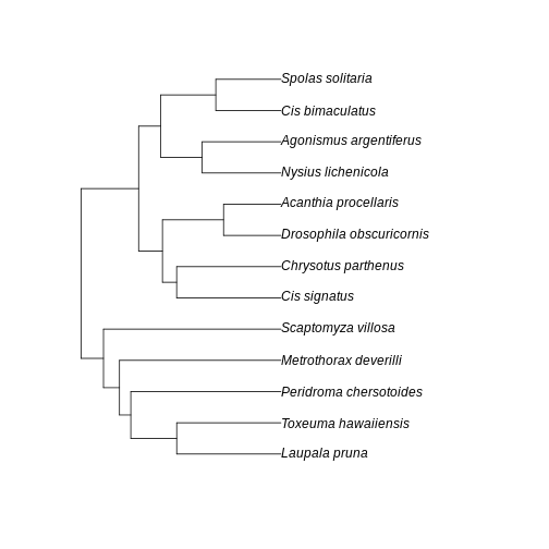
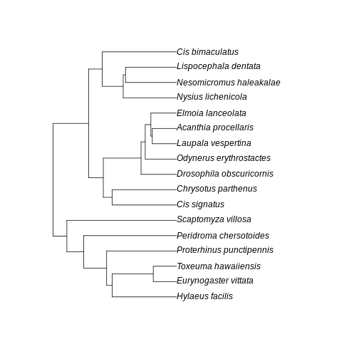
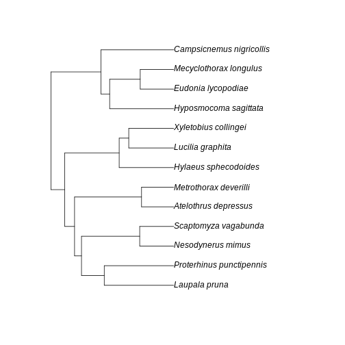
A few points of discussion: 1. Kauai has lowest absolute sum of branch lengths whereas Maui has the highest. The Big Island stays in between. 2. The Big Island, however, has the most uneven distribution of branch length. Even though branches are overall longer in the Big Island than in the Kauai island, lower Hill number on higher orders suggest they are more unevenly distributed in the community of the Big Island. 3. Lower values for the Big Island in higher orders, coupled with a slightly higher value for order 0, suggest that the evolutionary branches in this island are longer than in Kauai but they are unevenly represented, probably represented by a few very abundant species. This suggests a young history of colonization for this island: the community is dominated by the few good colonizers, which have been evolving for a while in the mainland, bring their long branches to the community when they arrive. The absence of shorter branches evenly distributed further suggests that speciation has not occurred much in this island, indicating a young community mostly composed by colonizers. 4. Kauai has the lowest sum of branch lengths, but evenness seems to be in between the other two islands. This suggests this islands harbors more closely related taxa (lowest sum of branches) when compared to other islands, but these values are evenly distributed among species. A longer history may be inferred here, with a lot of local speciation (accounting for closely related taxa) and probably competitive coexistence dictating similar abundances across species (accounting for evenness of branch representation). 5. Maui has overall highest PD in all orders and higher evenness of distribution of branch lengths. This suggests an intermediate history: both speciation and immigration account for a lot of evolutionary history in this island, while elapsed time may have been enough to dictate a more even distribution of species abundance and phylogenetic history.
Further visualization of the trees for each community can help us corroborate these ideas:
R
BI_tree <- keep.tip(arthro_tree_pruned,abundances$final_name[ abundances$island == 'BigIsland' ])
MA_tree <- keep.tip(arthro_tree_pruned,abundances$final_name[ abundances$island == 'Maui' ])
KA_tree <- keep.tip(arthro_tree_pruned,abundances$final_name[ abundances$island == 'Kauai' ])

plot(BI_tree)

R
plot(MA_tree)

R
plot(KA_tree)

The interesting thing here is that we could infer the history of the communities from the numbers only, before looking at the trees per community. This speaks to the power of Hill numbers as summary statistic of biodiversity patterns and how they can be useful for simulation-based inference.
Working with population genetic dataIntroductionWork with pop gen dataExtra
Finding multi-dimensional biodiversity dataSources of multidimensional biodiversity data: large open-access databasesSources of MDBD: Databases without APIsSources of MDBD: “small data” attached to papersRecap
Instructor Note
You will be prompted to get an ENTREZ API key. This is a good idea to do in order to make larger queries, but it won’t be necessary for this workshop.
Instructor Note
Time-permitting, this could be an opportunity for a 15-minute breakout exercise where individuals or groups pick a database or website and search for data, then report back on what they found and what the process was like.
CARE Principles and Data Repositories
Instructor Note
Guide learners toward metadata standards to transition to next section
