12 ML parameter estimation with MESS simulations
12.1 Key questions
- How do I estimate parameter values for continuous MESS model parameters?
- How do I evaluate the uncertainty of ML parameter estimates?
12.2 Lesson objectives
After this lesson, learners should be able to…
- Use simulations and randomForest ML to perform parameter estimation for key MESS model parameters.
- Evaluate uncertainty in parameter estimation accuracy using cross-validation simulations.
- Apply ML parameter estimation to empirical data and interpret results in terms of story
- Brainstorm applications to real data
12.3 Planned exercises
- Motivating MESS process-model parameter estimation
- Implement ML parameter estimation
- Hands-on Exercise: Predicting MESS parameters of mystery simulations
- Posterior predictive simulations (if time)
12.3.1 Motivating MESS process-model parameter estimation
Now that we have identified the neutral model as the most probable, we can estimate parameters of the emipirical data given this model. Essentially, we are asking the question “What are the parameters of the model that generate summary statistics most similar to those of the empirical data?”
12.3.2 Implement ML parameter estimation
Let’s start with a new clean Rscript, so create a new file and save it as “MESS-Regression.R”, then load the necessary libraries and simulated data.
12.3.2.1 Load libraries, setwd, and load the simulated data
library(randomForest)
library(caret)
library(reticulate)

setwd("/home/rstudio/MESS-inference")
simdata = MESS$load_local_sims("MESS-SIMOUT.csv")[[1]]
12.3.2.2 Extract sumulations generated under the ‘filtering’ assembly model
Let’s pretend that the most probable model from the classification procedure was ‘environmental filtering’. If our goal is to estimate parameters under this model then we want to exclude simulations from the ml inference that do not fit our most probable model. This can be achieved by selecting rows in the simdata data.frame that have “filtering” as the assembly_model.
simdata = simdata[simdata$assembly_model == "filtering", ]
simdata
12.3.2.3 Split train and test data as normal
Again, we’ll split the data into training and testing sets.
tmp <- sample(2, nrow(simdata), replace = TRUE, prob = c(0.7, 0.3))
train <- simdata[tmp==1,]
test <- simdata[tmp==2,]
12.3.2.4 Train the ML regressor as normal
Train the ml model to perform regression, as our focal dependent variable takes continuous values. The randomForest package auto-detects if the dependent variable is continuous or categorical, so there’s nothing more to do there. We will use the same formula as before, specifying local_S and the first Hill number on each axis of biodiversity as the predictor variables.
rf <- randomForest(colrate ~ local_S + pi_h1 + abund_h1 + trait_h1, data=train, proximity=TRUE)
rf
12.3.2.5 Plot results of predictions for colrate of held-out training set
For a regression analysis we can’t use a confusion matrix because the response is continuous, so instead we evaluate prediction accuracy by making a scatter plot showing predictions as a function of known simulated values. With perfect prediction accuracy the points in the scatter plot would fall along the identity line.
preds <- predict(rf, test)
plot(preds, test$colrate)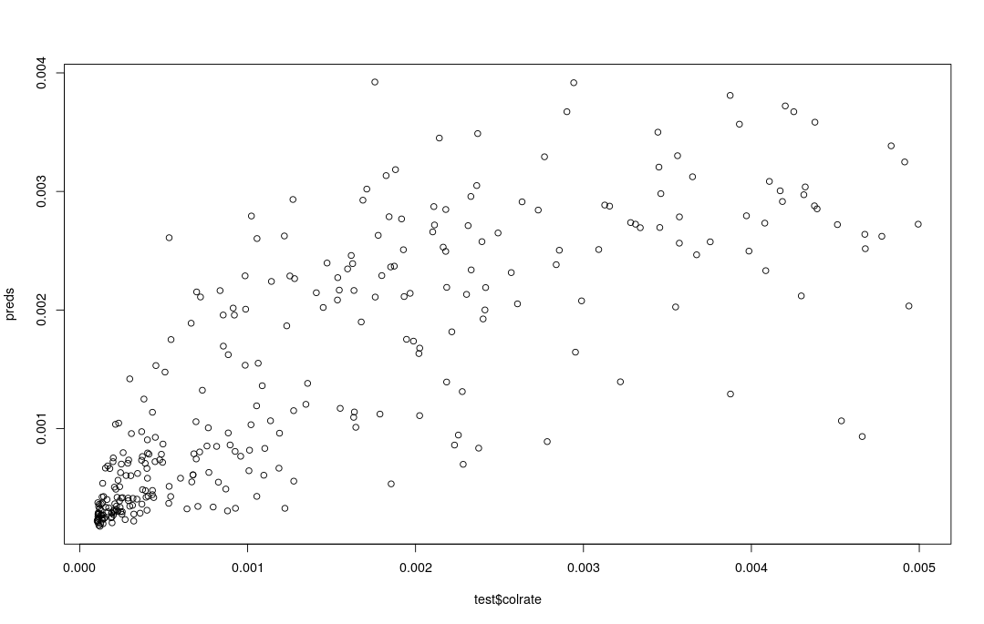
What we are doing here is a very qualitative, ad hoc evaluation of prediction accuracy. This is another case where the full details of performing ml inference are slightly out of scope for this workshop, given the amount of time we have. In a real analysis one should more formally quantify this with mean squared error, or mean absolute error, or pseudo-R^2, some of which are provided in the randomForest package, e.g.:
rf <- randomForest(colrate ~ local_S + pi_h1 + abund_h1 + trait_h1, data=train, proximity=TRUE)
mean(rf$rsq)0.621940112.3.2.6 Predict colrate of test simulation and plot distribution of predictions
Now we can practice making predictions for a single simulation and looking at uncertainty in the prediction. Like we did before we can select one simulation by using the test [#, ] row selection strategy on our test data.frame.
When we ask for predict.all=TRUE this will return the prediction value for each tree in the rf, and we can plot the aggregation of these predictions using hist to show a histogram.
predict() for regression
When predict.all=TRUE the predict() function returns a list with 2 elements:
- The predicted value (point estimate)
- A vector of predicted values for each tree in the forest
preds <- predict(rf, test[2, ], predict.all=TRUE)
# The predicted value is element [[1]]
print(preds[[1]])
# A vector of predictions for each tree in the forest [[2]]
hist(preds[[2]])
0.001191852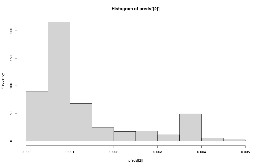
What can we say about the uncertainty on parameter estimation for this one simulation?
12.3.3 Hands-on Exercise: Predicting MESS parameters of mystery simulations
Now see if you can load the mystery simulations and do the regression inference on one or a couple of them. Try to do this on your own, but if you get stuck you can check the hint here:
## Importing the mystery data
mystery_sims = read.csv("/home/rstudio/MESS-inference/Mystery-data.csv")

## Predict for mystery sim 1
myst_sim = 1
mystery_pred = predict(rf, mystery_sims[myst_sim, ])
print(mystery_pred)
A link to the key containing the true colrate values is hidden below. Don’t peek until you have a guess for your simulated data! How close did you get?
If you are ahead of the group you will see that the “key” also contains the true values of J and ecological_strength so you might try performing the regression inference on these as well. Are either of these parameters harder or easier to estimate than colrate? Why do you think that is?
You might also try manipulating the predictor variables before training the ml model and evaluating the impact on performance. For example, try only using abundance Hill numbers, or only genetics Hill numbers. Try using all the Hill numbers for all the data axes. How does the composition of the predictor variables change the ml parameter estimation accuracy?
12.3.4 Posterior predictive simulations (if time)
Posterior predictive simulations are a good practice to assess the goodness of fit of the model to the data. Essentially this involves running new simulations setting MESS model parameters to the most probable estimates from the ML inference, and then evaluating the fit of the new simulations to the empirical data, typically by projecting summary statistics of the simulated and observed data and checking that they all fall within a point cloud.
We probably won’t have time to get to this, but it’s a good practice in fitting ml models to real data.
12.4 Key points
- Machine learning models can be used to “estimate parameters” of continuous response variables given multi-dimensional input data.
- Major components of machine learning inference include gathering and transforming data, splitting data into training and testing sets, training the ml model, and evaluating model performance.
- ML inference is inherently uncertain, so it is important to evaluate uncertainty in ml prediction accuracy and propagate this into any downstream interpretation when applying ml to empirical data.