Abundance Data
Last updated on 2023-07-11 | Edit this page
Overview
Questions
- What is abundance data, and how can we use it to gain insights about a system?
- How do I clean and manipulate abundance data to prepare for analyses?
- How do I calculate summary statistics and relate these to ecological pattern?
Objectives
After following this episode, participants should be able to…
- Describe ecological abundance data and what it can tell us about a system
- Import and examine organismal abundance data from .csv files
- Clean taxonomic names
- Manipulate abundance data into different formats
- Generate species abundance distribution plots from abundance data
- Summarize species abundance data using Hill numbers
- Interpret how different Hill numbers correspond to different signatures of species diversity
Introduction to abundance data
Abundance data is one of the most widely-collected biodiversity data types. It generally keeps track of how many individuals of each species (or taxonomic unit) are present at a site. It may also be recorded as relative abundances or percent cover, depending on the group.
There’s a huge diversity of applications of abundance data. Here, we’ll focus on one of the most generally-applicable approaches, which is to look at the diversity of a system. By diversity, we mean how abundance is distributed among the different taxonomic groups present in that system. This incorporates both species richness, and the evenness of how abundances is portioned among different species.
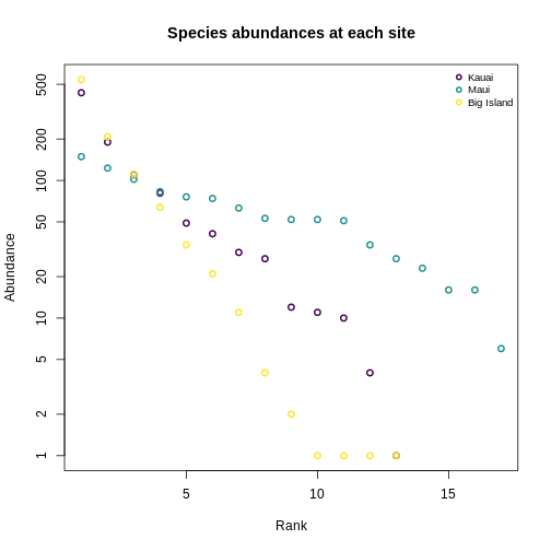
Let’s make this more concrete. If we plot the abundances of all the species in a system, sorted from most to least abundant, we end up with something like this:
This is the species abundance distribution, or SAD.
The SAD can show how even or uneven our system is.
Ok, great. What if we want to make comparisons between different systems? For that we need a quantifiable metric.
There are dozens - literally - of summary statistics for ecological diversity.
For this workshop, we’re going to focus on Hill numbers.
Hill numbers are a family of diversity indices that can be described verbally as the “effective number of species”. That is, they describe how many species of equal abundances would be present in a system to generate the corresponding diversity index.
Hill numbers are similar to other diversity indices you might have encountered. In fact, they mathematically converge with Shannon, Simpson, and species evenness.
Working with abundance data
Ok, so how about we do some actual coding?
For this episode, we’ll be working with a couple of specialized packages for biological data.
R
library(dplyr)
library(taxize)
library(hillR)
library(vegan)
library(tidyr)
Loading data
We’ll be working with ecological species abundance data stored in
.csv files. For help working with other storage formats, the
Carpentries’ Ecological Data lesson materials on databases are a
great place to start!
Let’s load the data:
R
abundances <- read.csv("https://raw.githubusercontent.com/role-model/multidim-biodiv-data/main/episodes/data/abundances_raw.csv")
And look at what we’ve got:
R
head(abundances)
OUTPUT
     island  site                GenSp abundance
1 BigIsland BI_01         Cis signatus       541
2 BigIsland BI_01 Acanthia procellaris        64
3 BigIsland BI_01     Spoles solitaria        34
4 BigIsland BI_01        Laupala pruna        21
5 BigIsland BI_01  Toxeuma hawaiiensis       111
6 BigIsland BI_01  Chrysotus parthenus       208
abundances is a data frame with columns for
island, site, GenSp, and
abundance. Each row tells us how many individuals of each
species (GenSp) were recorded at a given site on each island. This is a
common format - imagine you are censusing a plant quadrat, counting up
how many individuals of each species you see.
Cleaning taxonomic names
The first thing we’ll want to do is check for human error wherever we can, in this case in the form of typos in data entry.
The taxize R package can help identify and resolve
simple typos in taxonomic names.
R
species_list <- abundances$GenSp

name_resolve <- gnr_resolve(species_list, best_match_only = TRUE,
                            canonical = TRUE) # returns only name, not authority
R
head(name_resolve)
OUTPUT
# A tibble: 6 × 5
  user_supplied_name   submitted_name      data_source_title score matched_name2
  <chr>                <chr>               <chr>             <dbl> <chr>
1 Cis signatus         Cis signatus        Encyclopedia of … 0.988 Cis signatus
2 Acanthia procellaris Acanthia procellar… uBio NameBank     0.988 Acanthia pro…
3 Spoles solitaria     Spoles solitaria    Catalogue of Lif… 0.75  Spolas solit…
4 Laupala pruna        Laupala pruna       National Center … 0.988 Laupala pruna
5 Toxeuma hawaiiensis  Toxeuma hawaiiensis Encyclopedia of … 0.988 Toxeuma hawa…
6 Chrysotus parthenus  Chrysotus parthenus Encyclopedia of … 0.988 Chrysotus pa…
R
mismatches <- name_resolve[ name_resolve$matched_name2 !=
                                name_resolve$user_supplied_name, ]

mismatches[, c("user_supplied_name", "matched_name2")]
OUTPUT
# A tibble: 6 × 2
  user_supplied_name       matched_name2
  <chr>                    <chr>
1 Spoles solitaria         Spolas solitaria
2 Metrothorax deverilli    Metrothorax
3 Agonosmus argentiferus   Agonismus argentiferus
4 Agrotis chersotoides     Agrotis
5 Proterhenus punctipennis Proterhinus punctipennis
6 Elmoea lanceolata        Elmoia lanceolata
Four of these are just typos. But Agrotis chersotoides
in our data is resolved only to Agrotis and
Metrothorax deverilli is resolved to
Metrothorax. What’s up there?
R
name_resolve$matched_name2[
    name_resolve$user_supplied_name == "Agrotis chersotoides"] <-
    "Peridroma chersotoides"

name_resolve$matched_name2[
    name_resolve$user_supplied_name == "Metrothorax deverilli"] <-
    "Metrothorax deverilli"
Now we need to add the newly-resolved names to our
abundances data. For this, we’ll use a function called
left_join.
R
abundances <- left_join(abundances, name_resolve, by = c("GenSp" = "user_supplied_name"))

abundances$final_name <- abundances$matched_name2

head(abundances)
OUTPUT
     island  site                GenSp abundance       submitted_name
1 BigIsland BI_01         Cis signatus       541         Cis signatus
2 BigIsland BI_01 Acanthia procellaris        64 Acanthia procellaris
3 BigIsland BI_01     Spoles solitaria        34     Spoles solitaria
4 BigIsland BI_01        Laupala pruna        21        Laupala pruna
5 BigIsland BI_01  Toxeuma hawaiiensis       111  Toxeuma hawaiiensis
6 BigIsland BI_01  Chrysotus parthenus       208  Chrysotus parthenus
                              data_source_title score        matched_name2
1                          Encyclopedia of Life 0.988         Cis signatus
2                                 uBio NameBank 0.988 Acanthia procellaris
3                   Catalogue of Life Checklist 0.750     Spolas solitaria
4 National Center for Biotechnology Information 0.988        Laupala pruna
5                          Encyclopedia of Life 0.988  Toxeuma hawaiiensis
6                          Encyclopedia of Life 0.988  Chrysotus parthenus
            final_name
1         Cis signatus
2 Acanthia procellaris
3     Spolas solitaria
4        Laupala pruna
5  Toxeuma hawaiiensis
6  Chrysotus parthenus
Visualizing species abundance distributions
Now that we have cleaned data, we can generate plots of how abundance is distributed.
Because we’ll want to look at each island separately, we’ll use the
split command to break the abundances data
frame apart by island. split will split a dataframe into
groups defined by the f argument (for “factor”) - in this
case, the different values of the island column of the
abundances data frame:
R
island_abundances <- split(abundances, f = abundances$island)
Usual practice is to plot distributions of abundance as the species abundance on the y-axis and the rank of that species (from most-to-least-abundant) on the x-axis. This allows us to make comparisons between sites that don’t have any species in common.
Now, we’ll construct a plot with lines for the abundances of species on each island.
R
# figure out max number of species at a site for axis limit setting below
max_sp <- sapply(island_abundances, nrow)
max_sp <- max(max_sp)

plot(
    sort(island_abundances$Kauai$abundance, decreasing = TRUE),
    main = "Species abundances at each site",
    xlab = "Rank",
    ylab = "Abundance",
    lwd = 2,
    col = "#440154FF",
    xlim = c(1, max_sp),
    ylim = c(1, max(abundances$abundance)),
    log = 'y'
)

points(
    sort(island_abundances$Maui$abundance, decreasing = T),
    lwd = 2,
    col = "#21908CFF"
)

points(
    sort(island_abundances$BigIsland$abundance, decreasing = T),
    lwd = 2,
    col = "#FDE725FF"
)

legend(
    "topright",
    legend = c("Kauai", "Maui", "Big Island"),
    pch = 1,
    pt.lwd = 2,
    col = c("#440154FF", "#21908CFF", "#FDE725FF"),
    bty = "n",
    cex = 0.8
)

Quantifying diversity using Hill numbers
Let’s calculate Hill numbers to put some numbers to these shapes.
For this, we’ll need what’s known as a site by species matrix. This is a very common data format for ecological diversity data.
Site-by-species matrix
A site by species sites as rows and species as columns. We can get
there using the pivot_wider function from the package
tidyr:
R
abundances_wide <- pivot_wider(abundances, id_cols = site,
                              names_from = final_name,
                              values_from = abundance,
                              values_fill = 0)

head(abundances_wide[,1:10])
OUTPUT
# A tibble: 3 × 10
  site  `Cis signatus` `Acanthia procellaris` `Spolas solitaria` `Laupala pruna`
  <chr>          <int>                  <int>              <int>           <int>
1 BI_01            541                     64                 34              21
2 MA_01             52                     53                  0               0
3 KA_01              0                      0                  0              12
# ℹ 5 more variables: `Toxeuma hawaiiensis` <int>, `Chrysotus parthenus` <int>,
#   `Metrothorax deverilli` <int>, `Drosophila obscuricornis` <int>,
#   `Cis bimaculatus` <int>
We’ll want this data to have row names based on the sites, so we’ll need some more steps:
R
abundances_wide <- as.data.frame(abundances_wide)

row.names(abundances_wide) <- abundances_wide$site

abundances_wide <- abundances_wide[, -1]

head(abundances_wide)
OUTPUT
      Cis signatus Acanthia procellaris Spolas solitaria Laupala pruna
BI_01          541                   64               34            21
MA_01           52                   53                0             0
KA_01            0                    0                0            12
      Toxeuma hawaiiensis Chrysotus parthenus Metrothorax deverilli
BI_01                 111                 208                    11
MA_01                 102                  27                     0
KA_01                   0                   0                   190
      Drosophila obscuricornis Cis bimaculatus Nysius lichenicola
BI_01                        2               4                  1
MA_01                       83             149                 16
KA_01                        0               0                  0
      Agonismus argentiferus Peridroma chersotoides Scaptomyza villosa
BI_01                      1                      1                  1
MA_01                      0                     23                 63
KA_01                      0                      0                  0
      Lispocephala dentata Hylaeus facilis Laupala vespertina
BI_01                    0               0                  0
MA_01                  123              74                 52
KA_01                    0               0                  0
      Proterhinus punctipennis Nesomicromus haleakalae Odynerus erythrostactes
BI_01                        0                       0                       0
MA_01                       51                      76                      34
KA_01                      434                       0                       0
      Eurynogaster vittata Elmoia lanceolata Xyletobius collingei
BI_01                    0                 0                    0
MA_01                    6                16                    0
KA_01                    0                 0                   41
      Nesodynerus mimus Scaptomyza vagabunda Lucilia graphita
BI_01                 0                    0                0
MA_01                 0                    0                0
KA_01                30                   81               49
      Eudonia lycopodiae Atelothrus depressus Mecyclothorax longulus
BI_01                  0                    0                      0
MA_01                  0                    0                      0
KA_01                110                   10                     11
      Hylaeus sphecodoides Hyposmocoma sagittata Campsicnemus nigricollis
BI_01                    0                     0                        0
MA_01                    0                     0                        0
KA_01                    4                    27                        1
Let’s write it to a file in case we need to load it again later on:
R
write.csv(abundances_wide, here::here("episodes", "data", "abundances_wide.csv"), row.names = F)
WARNING
Warning in file(file, ifelse(append, "a", "w")): cannot open file
'/home/runner/work/multidim-biodiv-data/multidim-biodiv-data/site/built/episodes/data/abundances_wide.csv':
No such file or directory
ERROR
Error in file(file, ifelse(append, "a", "w")): cannot open the connectionCalculating Hill numbers with hillR
The hillR package allows us to calculate Hill
numbers.
R
hill_0 <- hill_taxa(abundances_wide, q = 0)

hill_0
OUTPUT
BI_01 MA_01 KA_01
   13    17    13
R
hill_1 <- hill_taxa(abundances_wide, q = 1)

hill_1
OUTPUT
    BI_01     MA_01     KA_01
4.001789 13.746057 5.949875 R
hill_2 <- hill_taxa(abundances_wide, q = 2)

hill_2
OUTPUT
    BI_01     MA_01     KA_01
 2.824029 11.958289  4.012680
Relating Hill numbers to patterns in diversity
Let’s revisit the SAD plots we generated before, and think about these in terms of Hill numbers.
R
plot(
    sort(island_abundances$Kauai$abundance, decreasing = TRUE),
    main = "Species abundances at each site",
    xlab = "Rank",
    ylab = "Abundance",
    lwd = 2,
    col = "#440154FF",
    xlim = c(1, max_sp),
    ylim = c(1, max(abundances$abundance)),
    log = 'y'
)

points(
    sort(island_abundances$Maui$abundance, decreasing = T),
    lwd = 2,
    col = "#21908CFF"
)

points(
    sort(island_abundances$BigIsland$abundance, decreasing = T),
    lwd = 2,
    col = "#FDE725FF"
)

legend(
    "topright",
    legend = c("Kauai", "Maui", "Big Island"),
    pch = 1,
    pt.lwd = 2,
    col = c("#440154FF", "#21908CFF", "#FDE725FF"),
    bty = "n",
    cex = 0.8
)
R
hill_abund <- data.frame(hill_abund_0 = hill_0,
                         hill_abund_1 = hill_1,
                         hill_abund_2 = hill_2)
hill_abund <- cbind(site = rownames(hill_abund), hill_abund)

rownames(hill_abund) <- NULL

hill_abund
OUTPUT
   site hill_abund_0 hill_abund_1 hill_abund_2
1 BI_01           13     4.001789     2.824029
2 MA_01           17    13.746057    11.958289
3 KA_01           13     5.949875     4.012680
Recap
Keypoints
- Organismal abundance data are a fundamental data type for population and community ecology.
- The
taxisepackage can help with data cleaning, but quality checks are often ultimately dataset-specific. - The species abundance distribution (SAD) summarizes site-specific abundance information to facilitate cross-site or over-time comparisons.
- We can quantify the shape of the SAD using summary statistics. Specifically, Hill numbers provide a unified framework for describing the diversity of a system.