Summarizing phylogenetic data
Last updated on 2023-07-11 | Edit this page
Overview
Questions
- What biological information is stored in phylogenetic Hill numbers?
- How do you import and manipulate phylogeny data in R?
- What are the common phylogeny data formats?
- How do you visualize phylogenies in R?
- How do you calculate Hill numbers with phylogenetic data?
Objectives
After following this episode, participants will be able to:
- Identify key features of the Newick format
- Import and manipulate phylogenetic data in the R environment
- Visualize phylogenies
- Calculate and interpret phylogenetic Hill numbers
Introduction to phylogenetic data
In this episode, we will explore how to extract information from phylogenetic trees in order to complement our hypotheses and inferences about processes shaping biodiversity patterns. Phylogenetic trees have information about how the species in a taxonomic group are related to each other and how much relative evolutionary change has accumulated among them. Since local communities differ in their phylogenetic composition, this information can give insights on why communities are how they are.
The relative phylogenetic distance among species in a community as well as the distribution of the amount of evolutionary history (represented by the length of the branches in a phylogeny) are a result of different factors such as the age since the initial formation of the community and the rate of macroevolutionary processes such as speciation and extinction. For instance, young communities that are dominated by closely related species and show very short branch lengths may suggest a short history with few colonization events and high rates of local speciation; alternatively, if the same young communities harbor distantly related species with longer branch lengths, it may suggest that most of the local diversity was generated by speciation elsewhere followed by colonization events involving distantly related species. Coupled with information on ecological traits and rates of macroevolutionary processes, these patterns also allow to test for hypotheses regarding, for instance, ecological filtering or niche conservatism.
Summarizing this phylogenetic information (i.e., phylogenetic distance and distribution of branch lengths) is therefore important for inference. As we have seen in previous episodes, the use of Hill numbers is an informative approach to summarize biodiversity. In this episode, we will see how phylogenetic Hill numbers in different orders are able to capture information about 1) the total amount of evolutionary history in different communities; 2) how this history is relatively distributed across the community.
Working with phylogenetic data in R
Importing phylogenetic data
Several file formats exist to store phylogenetic information. The
most common formats are the Newick and Nexus
formats. Both these formats are plain text files storing different
levels of information about the taxa relationship and evolutionary
history. Newick files are the standard for representing
trees in a computer-readable form, as they can be extremely simple and
therefore do not take up much memory. Nexus file, on the
other hand, are composed by different blocks regarding different types
of information and can be used to store DNA alignments, phylogenetic
trees, pre-defined groupings of taxa, or everything at once. Since they
are a step ahead in complexity, we will stick with Newick
files for now.
Newick files store the information about the clades in a
tree by representing each clade within a set of parentheses. Sister
clades are separated by ,. The notation also requires us to
add the symbol ; to represent the end of the information
for that phylogenetic tree.
The basic structure of a tree in a Newick format is
therefore as follows:
((A,B),C);
The notation above indicates that: 1. we have three taxa in our tree,
named A, B and C; 2.
A and B form one clade (A,B); 3. the (A,B)
clade is sister to the C clade (we represent that by adding
another set of parentheses and a , separating (A,B) from
C).
In addition, Newick files can also store information on
the branch leading to it tip and node. We do that by adding
: after each tip/node.
((A:0.5,B:0.5):0.5,C:1);
The notation above indicates that: 1. the branches containing A and B have each a length = 0.5; 2. the branch that leads to the node connecting A and B also has length = 0.5; 3. the branch leading to C has length = 1.
The notation above is what we import into R to start working with and manipulating our phylogenetic tree. For that goal, we will use the ape package. Below, we are also loading a few other packages we’ll be using later on.
R
library(ape)
library(tidyr)
library(hillR)
To import our tree, we will be using the function
read.tree() from the ape package. In the case
of simple trees as the one above, we could directly create them within R
by giving that notation as a character value to this
function, using the text argument, as shown below:
R
example_tree <- read.tree(text = '((A:0.5,B:0.5):0.5,C:1);')
Now, we can visually inspect our tree using the plot()
function:
R
plot(example_tree)
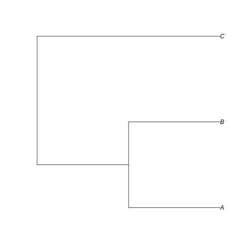
Can you visualize the text notation in that image? We can see the same information: A is closer related to B than C, and the branches leading to A and B have half the length of the branch leading to C.
The read.tree() function creates an object of class
phylo. We can further investigate this object by calling it
in our console:
R
example_tree
OUTPUT
Phylogenetic tree with 3 tips and 2 internal nodes.

Tip labels:
  A, B, C

Rooted; includes branch lengths.
The printed information shows us that we have a phylogenetic tree with 3 tips and 2 internal nodes, where the tip labels are “A, B, C”. We also are informed that this tree is rooted and has branch lengths.
One way to access the components of this object and better explore it
is to use $ after the object name. Here, it will be
important for us to know a little bit more about where the information
about tip labels and branch lengths are stored in that
phylo object. Easy enough, we can access that by calling
tip.labels and edge.length after
$.
R
example_tree$tip.label
OUTPUT
[1] "A" "B" "C"R
example_tree$edge.length
OUTPUT
[1] 0.5 0.5 0.5 1.0Cleaning and filtering phylogenetic data
Now that we learned how to import and visualize trees in R, let’s bring the phylogeny for the communities we are working with in this workshop. Our data so far consists of abundances and traits of several taxa of arthropods collected across three islands in the Hawaiian archipelago. Let’s work though importing phylogenetic information for these species.
Two common approaches to retrieving a phylogeny for a focal group are
1) relying on a published phylogeny for the group, or 2) surveying
public phylogenetic databases based on your taxa list. A common option
for the latter is the Open
Tree of Life Taxonomy, a public database that synthesizes taxonomic
information from different sources. You can even interact with this
database using the R package rotl. A few tutorials to do so
exist online, like this one.
Using a public database is a good approach when working with taxonomic
groups that are not heavily investigated regarding their phylogenetic
relationships (the well-known Darwinian
shortfall). In such cases, databases like OTL will give you a
summary phylogeny already filtered for the taxa you have in hand and
cross-checked for synonyms and misspellings.
For this workshop, since we are using simulated data, we will work
with the first option: a “published” arthropod phylogeny. Let’s load
this phylogeny into R using the function read.tree we
learned earlier.
R
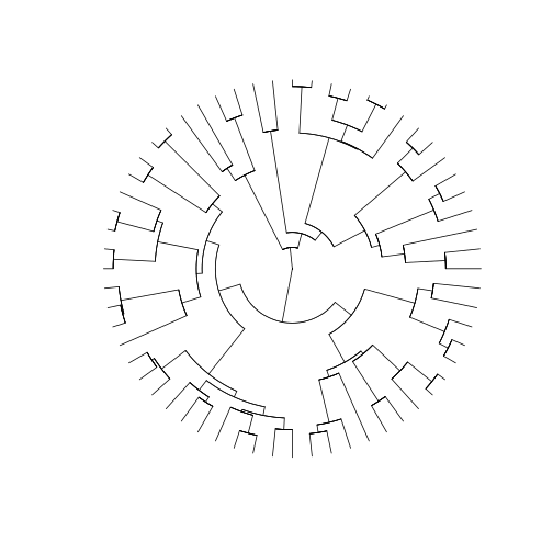
arthro_tree <- read.tree('https://raw.githubusercontent.com/role-model/multidim-biodiv-data/main/episodes/data/phylo_raw.nwk')

class(arthro_tree)
OUTPUT
[1] "phylo"This new phylo object is way larger than the previous
one, being a “real” phylogeny and all. You can inspect it again by
directly calling the object arthro_tree. To plot it, we
will use the type argument to modify how our tree will be
displayed. Here, we used the option 'fan', to display a
circular phylogeny (slightly better to show such a large phylogeny in
the screen). We also set the show.tip.label argument to
False.
R
plot(arthro_tree, type = 'fan', show.tip.label = F)
How do we combine all this information with the community datasets we have so far for our three islands? First, we will have to perform some name checking and filtering.
Cleaning and checking phylogeny taxa
The first thing we want to do is to check the tip labels in our tree. Since this is a “published” arthropod phylogeny, we will likely not have any misspelling in the tip names of the object. However, it is always good practice to check contents to see if anything weird stands out.
R
arthro_tree$tip.label
OUTPUT
 [1] "Leptogryllus_fusconotatus"   "Hylaeus_facilis"
 [3] "Laupala_pruna"               "Eurynogaster_vittata"
 [5] "Cydia_gypsograpta"           "Toxeuma_hawaiiensis"
 [7] "Proterhinus_punctipennis"    "Drosophila_quinqueramosa"
 [9] "Ectemnius_mandibularis"      "Nesodynerus_mimus"
[11] "Proterhinus_xanthoxyli"      "Nesiomiris_lineatus"
[13] "Aeletes_nepos"               "Scaptomyza_vagabunda"
[15] "Agrotis_chersotoides"        "Kauaiina_alakaii"
[17] "Atelothrus_depressus"        "Metrothorax_deverilli"
[19] "Scaptomyza_villosa"          "Hylaeus_sphecodoides"
[21] "Lucilia_graphita"            "Xyletobius_collingei"
[23] "Hyposmocoma_sagittata"       "Cis_signatus"
[25] "Hyposmocoma_scolopax"        "Dryophthorus_insignoides"
[27] "Eudonia_lycopodiae"          "Chrysotus_parthenus"
[29] "Limonia_sabroskyana"         "Hyposmocoma_marginenotata"
[31] "Mecyclothorax_longulus"      "Deinomimesa_haleakalae"
[33] "Trigonidium_paranoe"         "Eudonia_geraea"
[35] "Drosophila_furva"            "Hyposmocoma_geminella"
[37] "Drosophila_obscuricornis"    "Campsicnemus_nigricollis"
[39] "Odynerus_erythrostactes"     "Phaenopria_soror"
[41] "Gonioryctus_suavis"          "Laupala_vespertina"
[43] "Acanthia_procellaris"        "Odynerus_caenosus"
[45] "Elmoia_lanceolata"           "Nesodynerus_molokaiensis"
[47] "Sierola_celeris"             "Nysius_lichenicola"
[49] "Parandrita_molokaiae"        "Agonismus_argentiferus"
[51] "Cephalops_proditus"          "Nesomicromus_haleakalae"
[53] "Lispocephala_dentata"        "Agrion_nigrohamatum"
[55] "Plagithmysus_ilicis_ekeanus" "Scatella_clavipes"
[57] "Hedylepta_accepta"           "Cis_bimaculatus"
[59] "Hydriomena_roseata"          "Spolas_solitaria"
And indeed we find something: even though there are probably no
misspellings, the genus and species name in this tree are separated by
an underscore symbol _. Since the names in our
site-by-species matrix do not have that underscore, we will get an error
when matching the data if we don’t fix this spelling.
One useful function to do this fixing is the function
gsub(). This function allows you to look for a specific
character pattern inside character objects, and replace them by any
other pattern you may want. In our case, we have a vector of 60
character values containing the names of our tips. We want to find the
_ character inside each character value and replace it by
an empty space, so it becomes equal to what we have in our
site-by-species matrix. We do so by providing to the gsub()
function: 1) the pattern we want to replace; 2) the new pattern we want
to replace it with; 2) the character object or vector containing the
values to be searched. Finally, we assign the output of that function
back to the tip.label slot in the arthro_tree
object.
R
arthro_tree$tip.label <- gsub('_',' ',arthro_tree$tip.label)

# A quick check to see if worked
arthro_tree$tip.label
OUTPUT
 [1] "Leptogryllus fusconotatus"   "Hylaeus facilis"
 [3] "Laupala pruna"               "Eurynogaster vittata"
 [5] "Cydia gypsograpta"           "Toxeuma hawaiiensis"
 [7] "Proterhinus punctipennis"    "Drosophila quinqueramosa"
 [9] "Ectemnius mandibularis"      "Nesodynerus mimus"
[11] "Proterhinus xanthoxyli"      "Nesiomiris lineatus"
[13] "Aeletes nepos"               "Scaptomyza vagabunda"
[15] "Agrotis chersotoides"        "Kauaiina alakaii"
[17] "Atelothrus depressus"        "Metrothorax deverilli"
[19] "Scaptomyza villosa"          "Hylaeus sphecodoides"
[21] "Lucilia graphita"            "Xyletobius collingei"
[23] "Hyposmocoma sagittata"       "Cis signatus"
[25] "Hyposmocoma scolopax"        "Dryophthorus insignoides"
[27] "Eudonia lycopodiae"          "Chrysotus parthenus"
[29] "Limonia sabroskyana"         "Hyposmocoma marginenotata"
[31] "Mecyclothorax longulus"      "Deinomimesa haleakalae"
[33] "Trigonidium paranoe"         "Eudonia geraea"
[35] "Drosophila furva"            "Hyposmocoma geminella"
[37] "Drosophila obscuricornis"    "Campsicnemus nigricollis"
[39] "Odynerus erythrostactes"     "Phaenopria soror"
[41] "Gonioryctus suavis"          "Laupala vespertina"
[43] "Acanthia procellaris"        "Odynerus caenosus"
[45] "Elmoia lanceolata"           "Nesodynerus molokaiensis"
[47] "Sierola celeris"             "Nysius lichenicola"
[49] "Parandrita molokaiae"        "Agonismus argentiferus"
[51] "Cephalops proditus"          "Nesomicromus haleakalae"
[53] "Lispocephala dentata"        "Agrion nigrohamatum"
[55] "Plagithmysus ilicis ekeanus" "Scatella clavipes"
[57] "Hedylepta accepta"           "Cis bimaculatus"
[59] "Hydriomena roseata"          "Spolas solitaria"
Now that we fixed this first obvious issue, we can start looking for others. Since we want to calculate phylogenetic diversity for each of our communities, our main concern here is to make sure that all taxa present in our communities can be found in this phylogeny. One important issue that may arise is the use of different names for the same taxa across the two datasets (i.e., synonyms). This is especially important since we previouslu performed a synonym check and cleaning in our abundance dataset; we need to make sure the names in our tree will follow the same nomenclature decisions.
To see if there are any mismatches, let’s first retrieve a list of
the names in our abundances dataset. Since this dataset has repeated
instances of the same species when it shows up in different islands, we
wrap the vector of taxa names in the function unique() to
return each species name only once.
R
all_names <- unique(abundances$final_name)
To cross-check this list against the list of names in our phylogeny,
we can use the Boolean operator %in% coupled with
!. This will allow us to check for names present in
all_names that are not included in the
arthro_tree$tip.label. In summary, the expression
A %in% B would return whether each element of vector A is
present in vector B. This is returned as a Boolean vector: if
TRUE, the element of that position in A exists in B; if
FALSE, it does not. We add the ! (NOT)
operator to return the opposite of that expression, in a way that
!(A %in% B) will return whether each element of vector A is
NOT present in vector B. In this case, every time we see
TRUE, it means the element in that position is NOT
in vector B.
R
not_found <- !(all_names %in% (arthro_tree$tip.label))
not_found
OUTPUT
 [1] FALSE FALSE FALSE FALSE FALSE FALSE FALSE FALSE FALSE FALSE FALSE  TRUE
[13] FALSE FALSE FALSE FALSE FALSE FALSE FALSE FALSE FALSE FALSE FALSE FALSE
[25] FALSE FALSE FALSE FALSE FALSE FALSE FALSE
Checking the vector not_found, we can see it is a
collection of TRUEs and FALSEs. We can use that vector to perform
bracket subsetting in the vector all_names. Doing so, we
are retrieving from all_names only the elements in the
position where not_found is TRUE.
R
all_names[not_found]
OUTPUT
[1] "Peridroma chersotoides"The expression above give us the one element of
all_names that is not present in
arthro_tree$tip.label. As we expected, it is a synonym that
we corrected in our abundances
episode. Our tree still has the old name Agrotis chersotoides
whereas our site-by-species matrix has the updated name Peridroma
chersotoides. To correct that, we need to modify the tip label in
our tree to match the new name. How can we do that?
Challenge
Modify the old name Agrotis chersotoides in our phylogenetic tree, replacing it by Peridroma chersotoides. To do so, you will need to 1) find the position of the old name in labels in our tree; 2) assign the new name in the right position where the old name is.
Hint: a similar task was performed before in the abundances.
We need to perform an assignment operation in the position where the
old name is located inside arthro_tree$tip.label. To find
that position, we can use Boolean matching to ask which element of
arthro_tree$tip.label equals the old name.
R
arthro_tree$tip.label[arthro_tree$tip.label == 'Agrotis chersotoides'] <- "Peridroma chersotoides"
A good practice after correcting the name is to re-check if all names
in our abundance dataset match the names in the phylogeny. This time, we
expect all elements in the vector not_found to be
FALSE. We can use the function which() to ask
“which elements in not_found are TRUE We
expect the answer to be an empty vector, indicating”no elements in
not_found are TRUE“.
R
not_found <- !(all_names %in% (arthro_tree$tip.label))
which(not_found)
OUTPUT
integer(0)Pruning our phylogeny
Now that we have a modified tree where all taxa names are present in our abundances dataset, we can work on pruning our phylogeny to the taxa present in our communities. This is especially important when working with published phylogenies as these are usually large files containing several taxa that may not exist in the local community.
We can prune our phylogeny using the function keep.tip()
from the ape package. For this function, we provide the
entire phylogeny plus the names of the tips we want to keep. Here, we
will retrieve those names from the abundances dataset.
R
arthro_tree_pruned <- keep.tip(arthro_tree,abundances$final_name)
With a pruned phylogeny and a site-by-species matrix, we have the two bits of information we need to summarize phylogenetic diversity per community. As we saw in previous episodes, we can use such abundance matrix to calculate Hill numbers and help us compare patterns across the different communities. In the traits episode, we saw how we can combine abundance and trait data to extract Hill numbers as values that summarize the distribution of trait variation across communities. Here we will be following the same approach to summarize the amount and the distribution of evolutionary history across the species in our community.
Summarizing with hill numbers
In this section, we will extract some summary statistics about the pattern of phylogenetic diversity (PD) in our communities. As we discussed in the intro of this episode, the relative phylogenetic distance among species and the distribution of this distance can give insights into processes of community assembly. Here, we will make use of Hill numbers to extract summaries of phylogenetic distances, i.e. the length of the branches in the phylogenetic tree leading to the taxa present in each community. Phylogenetic hill numbers incorporate information on both the phylogenetic structure of a system and the abundances of different species. In order to get an intuition for how these different components influence phylogenetic hill numbers, we’ll set our Hawaiian data aside for a moment and first explore the behavior of this summary statistic using a few simplified example datasets.
Example 1. Trees with different branch lenghts
For our examples, we’ll assume we have one single community with
eight taxa: A through H. Let’s create two site-by-species matrix for
this community: one denoting even abundance across species, and another
one with uneven abundance. For the even communitu, we create a vector of
the value 1 repeated 8 times; for the uneven community,
we’ll create a vector where abundance goes up from species A to species
H (for simplicity, we’ll just use values from 1 to 8). We then transform
them to dataframe, and name the columns with the names of the
species.
R
even_comm <- data.frame(rbind(rep(1,8))) # Abundance = 1 for all species
uneven_comm <- data.frame(rbind(seq(1,8))) # Abundance equal 1 for species A and goes up to 8 towards species H.

# We name the columns with the species names
colnames(even_comm) <- colnames(uneven_comm) <- c('A','B','C','D','E','F','G','H')
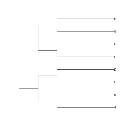
Now let’s create two different possible trees for these communities: one with short branch lengths and another with longer branch lengths. Remember: branch length = amount of evolutionary change
R
short_tree <- read.tree(text='(((A:3,B:3):1,(C:3,D:3):1):1,((E:3,F:3):1,(G:3,H:3):1):1);')
long_tree <- read.tree(text='(((A:6,B:6):1,(C:6,D:6):1):1,((E:6,F:6):1,(G:6,H:6):1):1);')
If we plot both trees…
R
plot(short_tree)
R
plot(long_tree)
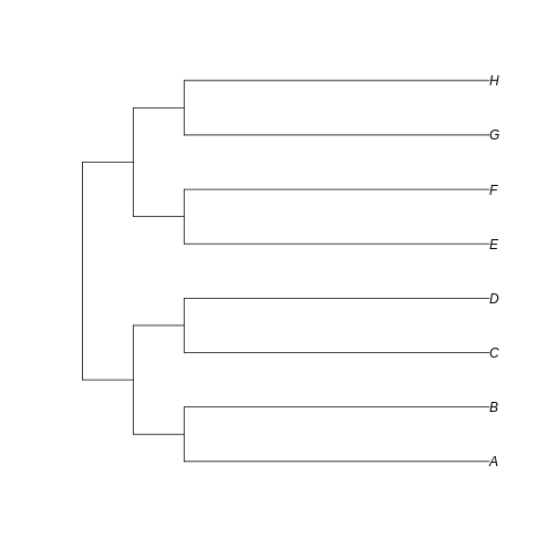
…we can see that the branches leading to extant taxa are longer for
long_tree, as we intended. This suggests that a greater
amount of evolutionary change is happening in these recent branches of
the longer tree when compared to the shorter tree.
Now, we will calculate phylogenetic hill numbers for both trees using
both even and uneven communities. To store the calculated values, we’ll
create a data.frame called even_comm_short_tree. The first
column will be our Hill numbers to be calculated; the second column will
be the Hill number order from 0 to 3, to see how the order affects the
values; the third and fourth column will be the description of our
components
R
even_comm_short_tree <- data.frame(
    hill_nb = NA,
    q = 0:3,
    comm = "even",
    tree = "short"
)
Now we will use a for loop to calculate phylogenetic
Hill numbers using the hill_phylo function from the
hillR package. This function takes in a a site-by-species
matrix and phylogeny, and returns phylogenetic Hill numbers for each
site based on which species are present there. We provide to the
function the site-by-species matrix, the phylogenetic tree and the
order.
R
for(i in 1:nrow(even_comm_short_tree)) {
    even_comm_short_tree$hill_nb[i] <- hill_phylo(even_comm, short_tree, q = even_comm_short_tree$q[i])
}
Let’s repeat this process for the longer tree:
R
even_comm_long_tree <- data.frame(
    hill_nb = NA,
    q = 0:3,
    comm = "even",
    tree = "long"
)

for(i in 1:nrow(even_comm_long_tree)) {
    even_comm_long_tree$hill_nb[i] <- hill_phylo(even_comm, long_tree, q = even_comm_long_tree$q[i])
}
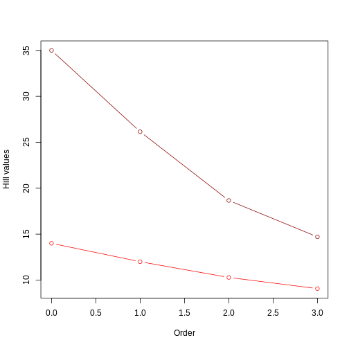
We can combine both dataframes and plot the values for comparison:
R
even_comm_nb <- data.frame(rbind(even_comm_short_tree,even_comm_long_tree))

plot(even_comm_nb$q[even_comm_nb$tree=='short'],
     even_comm_nb$hill_nb[even_comm_nb$tree=='short'],
     type='b',col='red',
     xlab = 'Order',ylab='Hill values',
     xlim = range(even_comm_nb$q),
     ylim = range(even_comm_nb$hill_nb))

lines(even_comm_nb$q[even_comm_nb$tree=='long'],
     even_comm_nb$hill_nb[even_comm_nb$tree=='long'],
     type='b',col='darkred')
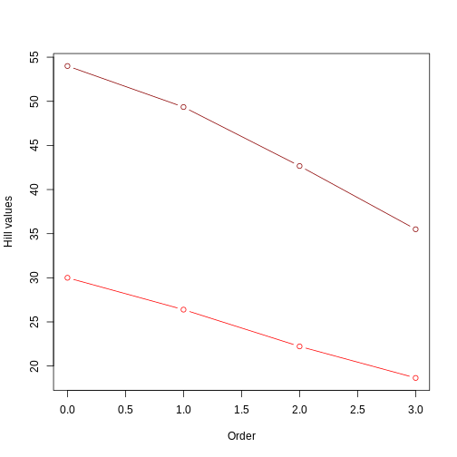
This figure clearly shows that the tree with longer branches (dark red line) harbors higher evolutionary history, and therefore higher PD, as calculated by Hill numbers. It also shows that the Hill number value decreases as the order goes up, since higher orders focus on branch lengths that are more common.
What would happen if the abundance of species in our community was uneven (a more realistic scenario)? In this case, both branch lengths and how abundant each branch is will have an effect on the calculated value. To visualize, let’s repeat the calculations above for the uneven community.
R
# Uneven comm with short tree
uneven_comm_short_tree <- data.frame(
    hill_nb = NA,
    q = 0:3,
    comm = "uneven",
    tree = "short"
)

for(i in 1:nrow(uneven_comm_short_tree)) {
    uneven_comm_short_tree$hill_nb[i] <- hill_phylo(uneven_comm, short_tree, q = uneven_comm_short_tree$q[i])
}

# Uneven comm with long tree
uneven_comm_long_tree <- data.frame(
    hill_nb = NA,
    q = 0:3,
    comm = "uneven",
    tree = "long"
)

for(i in 1:nrow(uneven_comm_long_tree)) {
    uneven_comm_long_tree$hill_nb[i] <- hill_phylo(uneven_comm, long_tree, q = uneven_comm_long_tree$q[i])
}

# Combining results
uneven_comm_nb <- data.frame(rbind(uneven_comm_short_tree,uneven_comm_long_tree))
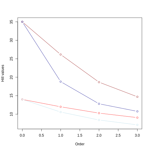
Let’s plot all results together, using red colors for even communities and blue colors for uneven community. Ligher colors will represent short trees whereas darker colors will represent long trees.
R
plot(even_comm_nb$q[even_comm_nb$tree=='short'],
     even_comm_nb$hill_nb[even_comm_nb$tree=='short'],
     type='b',col='red',
     xlab = 'Order',ylab='Hill values',
     xlim = range(even_comm_nb$q),
     ylim = range(min(uneven_comm_nb$hill_nb),max(even_comm_nb$hill_nb)))

lines(even_comm_nb$q[even_comm_nb$tree=='long'],
     even_comm_nb$hill_nb[even_comm_nb$tree=='long'],
     type='b',col='darkred')

lines(uneven_comm_nb$q[uneven_comm_nb$tree=='short'],
     uneven_comm_nb$hill_nb[uneven_comm_nb$tree=='short'],
     type='b',col='lightblue')

lines(uneven_comm_nb$q[uneven_comm_nb$tree=='long'],
     uneven_comm_nb$hill_nb[uneven_comm_nb$tree=='long'],
     type='b',col='darkblue')
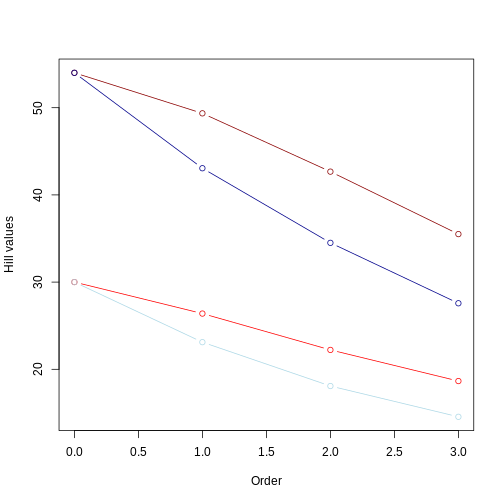
From this picture, we can take a few insights:
Longer branches still yield higher Hill numbers, regardless of the evenness in the community abundance;
The Hill number for q = 0 remains the same, regardless of the evenness.
As already observed, the value of the hill numbers drop as the order goes up. In the even community, since species have the same abundance, this decrease reflects higher orders focusing on more common values of branch lengths. In the uneven community, where species have different abundances, this decrease reflects higher orders focusing less and less on branches leading to rare taxa.
For q = 1 to 3, Hill numbers are always lower for uneven communities. This suggests that although branch lengths are the same (e.g., both dark red and dark blue lines represent the long tree), these branches are unevenly represented in the community due to uneven abundance of species. This unevenness is represented by the lower values of Hill number on higher orders. In other words, some branches in the tree “dominate” the community more than others. We can summarize this by saying that the higher the unevenness the lower the value of the Hill number will be.
Keypoints
-
hillRcalculates phylogenetic hill numbers given a phylogeny and a site by species matrix. - In trees with a similar topology, phylogenetic Hill number of order 0 reflect the sum of branch lengths. Orders of 1 and higher reflect the sum of branch lengths weighted by the relative abundance of different species.
Example 2. Balanced vs unbalanced trees
So far, we have learned that Hill numbers are affected by both the sum of branch lengths and the relative representation of each branch (in terms of species abundance) in the community. For example 1, we have used a perfectly balanced tree, i.e., all extant taxa have equal branch length. In example 2, we will explore the effects of the uneven distribution of cladogenesis event along the tree, leading to different phylogeny structures.
Let’s create a totally balanced tree…
R
balanced_tree <- read.tree(text='(((A:1,B:1):1,(C:1,D:1):1):1,((E:1,F:1):1,(G:1,H:1):1):1);')
… and a totally unbalanced tree.
R
unbalanced_tree <- read.tree(text='(A:7,(B:6,(C:5,(D:4,(E:3,(F:2,(G:1,H:1):1):1):1):1):1):1);')
Let’s plot both trees for comparison:
R
plot(balanced_tree)
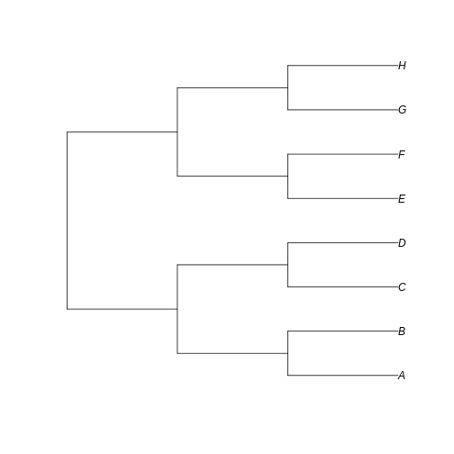
R
plot(unbalanced_tree)
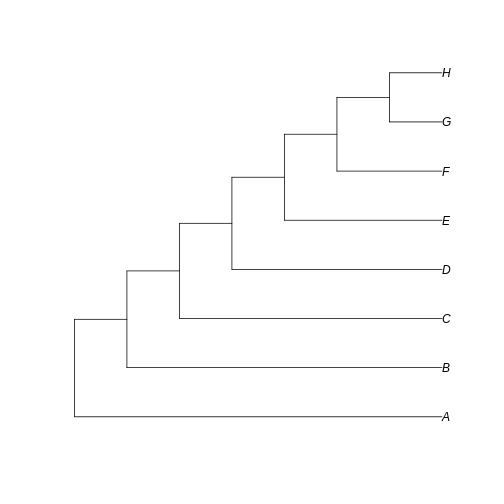
Notice that here the difference between the trees resides in the fate of each new lineage at a node. In the unbalanced uneven tree, at each diversification event one of the lineages always persists till the present with no change while the other undergoes another round of diversification. In the even tree, both lineages from each node undergo a new split. The consequence is that in the even tree, all extant species result from recent diversification (i.e., they have a short evolutionary history before coalescing into their ancestor), whereas in the unbalanced tree we have a mix of old and recent lineages. This means that the phylogenetic history itself is creating an uneven representation of branch lengths across the community (even before we account for species abundance)
To see how such phylogenetic structure influences hill numbers, let’s repeat the calculations from example 1 with these new trees. First, let’s focus on the even community (i.e., not introducing the relative species abundance factor yet):
R
even_comm_balanced_tree <- data.frame(
    hill_nb = NA,
    q = 0:3,
    comm = "even",
    tree = "balanced"
)

for(i in 1:nrow(even_comm_balanced_tree)) {
    even_comm_balanced_tree$hill_nb[i] <- hill_phylo(even_comm, balanced_tree, q = even_comm_balanced_tree$q[i])
}

even_comm_unbalanced_tree <- data.frame(
    hill_nb = NA,
    q = 0:3,
    comm = "even",
    tree = "unbalanced"
)

for(i in 1:nrow(even_comm_unbalanced_tree)) {
    even_comm_unbalanced_tree$hill_nb[i] <- hill_phylo(even_comm, unbalanced_tree, q = even_comm_unbalanced_tree$q[i])
}

even_comm_nb <- data.frame(rbind(even_comm_balanced_tree,even_comm_unbalanced_tree))

plot(even_comm_nb$q[even_comm_nb$tree=='balanced'],
     even_comm_nb$hill_nb[even_comm_nb$tree=='balanced'],
     type='b',col='red',
     xlab = 'Order',ylab='Hill values',
     xlim = range(even_comm_nb$q),
     ylim = range(even_comm_nb$hill_nb))

lines(even_comm_nb$q[even_comm_nb$tree=='unbalanced'],
     even_comm_nb$hill_nb[even_comm_nb$tree=='unbalanced'],
     type='b',col='darkred')
This plot is similar to example 1 in two ways: 1) one of the trees has higher hill number values, in this case the unbalanced tree. This suggests that the unbalanced structure of the tree accounts for a deeper evolutionary history (i.e., lineages have overall longer branches); 2) the value of the hill numbers drop as the order goes up. This happens because higher orders are weighting less and less those branch lengths that are not so common (like, for instance, the short branch lengths in the unbalanced tree).
Something new that we observe here is a more evident difference between trees in the rate of change of the Hill number value as we increase the order. The unbalanced tree (darker red) shows a steeper drop than the balanced tree (lighter red). This is similar to what we observed in the abundances episode: uneven communities show a steeper drop in Hill numbers as order increases. In this example, instead of species abundance, the unevenness of the community is represented by the structure of the phylogeny: a completely unbalanced tree combining long and short branches generates an unevenness in the distribution of branch lengths. Notice that this difference in rate of change barely observed in example 1: when plotting two trees with the same structure (short vs long trees, but both fully balanced), the lines are very similar In example 1, the difference in the rate of change only becomes evident when we incorporate unevenness from the species abundance, but here in example 2 we see this difference deriving already from the different structures of the trees.
If the tree structure is already introducing some unevenness in our community, how would the pattern differ when species relative abundance is included?
In this case, both the structure of the tree and the species abundance interact to generate a pattern of unevenness. Specifically, the overall value of PD will be the sum of branch lengths weighted by their abundance in the community as informed by the species abundance distribution (instead of by the frequency of the branch length in the tree). This added information brings new insights. It may be the case, for instance, that in the unbalanced tree, even though long branches are over represented, maybe the species with long branches are actually super rare in our community, and the short-branch species are actually super abundant. As you can probably infer, this difference suggests something about the evolutionary history of our community, in this case that the most abundant species have a very recent evolutionary history. Similarly, even though branch lengths are the same in the balanced tree, if some of the species is more abundant than others, it suggests that the evolutionary history of the tree is unevenly represented in our community.
To visualize these interaction between tree structure and species relative abundance, let’s redo the calculation for Hill numbers with balanced and unbalanced trees, this time using the uneven community. We’ll plot all final values together for comparison.
R
uneven_comm_balanced_tree <- data.frame(
    hill_nb = NA,
    q = 0:3,
    comm = "uneven",
    tree = "balanced"
)

for(i in 1:nrow(uneven_comm_balanced_tree)) {
    uneven_comm_balanced_tree$hill_nb[i] <- hill_phylo(uneven_comm, balanced_tree, q = uneven_comm_balanced_tree$q[i])
}

uneven_comm_unbalanced_tree <- data.frame(
    hill_nb = NA,
    q = 0:3,
    comm = "uneven",
    tree = "unbalanced"
)

for(i in 1:nrow(uneven_comm_unbalanced_tree)) {
    uneven_comm_unbalanced_tree$hill_nb[i] <- hill_phylo(uneven_comm, unbalanced_tree, q = uneven_comm_unbalanced_tree$q[i])
}

uneven_comm_nb <- data.frame(rbind(uneven_comm_balanced_tree,uneven_comm_unbalanced_tree))

plot(even_comm_nb$q[even_comm_nb$tree=='balanced'],
     even_comm_nb$hill_nb[even_comm_nb$tree=='balanced'],
     type='b',col='red',
     xlab = 'Order',ylab='Hill values',
     xlim = range(even_comm_nb$q),
     ylim = range(min(uneven_comm_nb$hill_nb),max(even_comm_nb$hill_nb)))

lines(even_comm_nb$q[even_comm_nb$tree=='unbalanced'],
     even_comm_nb$hill_nb[even_comm_nb$tree=='unbalanced'],
     type='b',col='darkred')

lines(uneven_comm_nb$q[uneven_comm_nb$tree=='balanced'],
     uneven_comm_nb$hill_nb[uneven_comm_nb$tree=='balanced'],
     type='b',col='lightblue')

lines(uneven_comm_nb$q[uneven_comm_nb$tree=='unbalanced'],
     uneven_comm_nb$hill_nb[uneven_comm_nb$tree=='unbalanced'],
     type='b',col='darkblue')
Reminders: 1) light colors represent balanced trees, whereas darker colors represent unbalanced trees 2) red lines represent even community whereas blue lines represent uneven community.
From this second plot, we notice that:
Hill number values for the unbalanced tree (darker colors) are still higher than those for the balanced tree (lighter colors). This makes sense since the relative abundance is the same for both trees, so the overall pattern (i.e., longer branches in unbalanced tree) remains;
the Hill number of order 0 is the same regardless of whether you have different relative abundances among species. This was also the case for example 1. Order 0 is simply the sum of all branch lengths (i.e., it does not account for the relative abundance of branch lengths or taxa);
the inclusion of an uneven community accentuates the rate of decrease in the Hill number value as we increase the order. This is because higher orders are now affected by the unevenness of the distribution of branch length as well by the unevenness of species abundance. This is a good example of how calculating different order of hill numbers while incorporating species abundance allows to have a couple summary statistics accounting for evolutionary history and species abundance distribution that is comparable across different regions.
Keypoints
- The phylogenetic structure of the community (represented by the topology of the tree) influences the evenness of the branch length distribution and contribute to different rates in the decrease of Hill number values as the order number increases.
- The inclusion of community structure (relative abundance of different species) further accentuates this difference in rate of change.
- Phylogenetic Hill numbers represent the sum of branch lenghts. Higher orders weight that sum by the distribution of branch lengths and the species relative abundance.
Now that we acquired an intuition on the information phylogenetic Hill numbers can give us, let’s move on to our actual data.
Moving on to our island communities
For this final section, we will be working on the data for the three island communities to calculate hill numbers from orders of 0 to 3. We will be using our pruned phylogeny and the site-by-species matrix we created in the abundances episode. Since we covered the workflow of calculating phylogenetic Hill numbers in the previous section, we will leave this activity for a challenge.
Challenge
For this challenge, you should calculate the phylogenetic Hill
numbers of orders 0 to 3 for the three islands we are working with
throughout the workshop The key objects here will be the phylogeny
stored in arthro_tree_pruned and the sites-by-species
matrix stored in abundances_wide. You should also plot the
hill numbers for each island and discuss what the calculated values
allow you to infer regarding the history of each community.
We can directly calculate Hill numbers using the
hill_phylo function along with the objects
arthro_tree_pruned and abundances_wide. Since
we have three sites, the function will return a vector with tree values,
one Hill number for each site of the order we requested. Let’s create an
empty list to store a vector for each order, and use a for
loop to calculate from orders of 0 to 3.
R
hill_values <- vector('list', length = 4)
for (i in 0:3) {
    hill_values[[i + 1]] <- hill_phylo(abundances_wide, arthro_tree_pruned,
                                       q = i)
}
Now, let’s create a data.frame with islands as rows and Hill numbers
of different orders as columns. For that, we will use the function
do.call to collapse our list hill_values using
the function cbind.
R
hill_values <- do.call(cbind.data.frame, hill_values)
colnames(hill_values) <- paste0('hill_phylo_', 0:3)
hill_phylo <- data.frame(site = rownames(hill_values),
                         hill_values)

rownames(hill_phylo) <- NULL
hill_phylo
OUTPUT
   site hill_phylo_0 hill_phylo_1 hill_phylo_2 hill_phylo_3
1 BI_01     59.09643     18.71926     13.41881     11.65893
2 MA_01     64.21265     40.30308     26.89875     20.36594
3 KA_01     54.49430     28.10458     20.00878     16.29594
Finally, we can plot using a similar code to the ones we used in our
examples. We set xlim to go from 0 to 3, and
ylim to go from the lowest to the highest value in the
object hill_values. We also add a legend using the
legend() function like we did in the traits episode.
R
plot(seq(0,3),hill_phylo_nbs[3,2:5],
     type='b',col="#440154FF",
     xlab = 'Order',ylab='Hill values',
     xlim = c(0,3),
     ylim = range(min(hill_values),max(hill_values)))
ERROR
Error in eval(expr, envir, enclos): object 'hill_phylo_nbs' not foundR
lines(seq(0,3),hill_phylo_nbs[2,2:5],
      type='b',col="#21908CFF")
ERROR
Error in eval(expr, envir, enclos): object 'hill_phylo_nbs' not foundR
lines(seq(0,3),hill_phylo_nbs[1,2:5],
      type='b',col="#FDE725FF")
ERROR
Error in eval(expr, envir, enclos): object 'hill_phylo_nbs' not foundR
legend(
    "topright",
    legend = c("Kauai","Maui","Big Island"),
    pch = 19,
    col = c("#440154FF", "#21908CFF", "#FDE725FF")
)
ERROR
Error in (function (s, units = "user", cex = NULL, font = NULL, vfont = NULL, : plot.new has not been called yetDiscussion
After calculating and plotting hill numbers, what inferences can you make about the history of these communities, in terms of the rates of local speciation and colonization?
Are there any further visualizations we haven’t done so far that you could make to further investigate the phylogenetic history of each community?