Finding multi-dimensional biodiversity data
Last updated on 2023-07-11 | Edit this page
Overview
Questions
- Where do multi-dimensional biodiversity data live online?
- How can we use R APIs to quickly and reproducibly retrieve data?
- What about data that’s not in a database?
Objectives
After following this episode, we intend that participants will be able to:
- Effectively search for and find occurrence, phylogenetic, sequence, and trait data online given a taxon or research question
- Retrieve data from NCBI & GBIF using their R APIs and apply API principles to other databases
Sources of multidimensional biodiversity data: large open-access databases
Large open-access biological databases have been growing at an incredible pace in recent years. Often they accumulate data from many projects and organizations. These platforms are then used to share and standardize data for wide use.
Many such databases exist, but here are some listed examples:
GBIF contains occurrence records of individuals assembled from dozens of smaller databases.
NCBI (National Center for Biotechnology Information) database, which includes GenBank is the largest repository of genetic data in the world, but includes a lot of biomedical data.
OTOL (Open Tree of Life) is a database that combines numerous published trees and taxonomies into one supertree
GEOME (Genomic Observatories MetaDatabase) contains genetic data associated with specimens or samples from the field.
BOLD (Barcode of Life) is a reference library and database for DNA barcoding
EOL (Encyclopedia of Life) is a species-level platform containing data like taxonomic descriptions, distribution maps, and images
What’s an API?
An API is a set of tools that allows users to interact with a database, such as reading, writing, updating, and deleting data. We can’t go over all of these databases in detail, but let’s cover some examples that illustrate some principles of how these APIs work for different types of biodiversity data.
We can do this using the example of Hawaiian arthropods. Hawaii is known for its diversity of Tetragnatha, a genus of orb weaver spiders. With this target in mind let’s download some occurrence data from GBIF, some sequence data from NCBI, and a phylogeny for Tetragnatha spiders from OTOL.
Using APIs: Setup
For this episode, we’ll be working with some R packages that wrap the APIs of online repositories. Let’s set those up now.
R
library(spocc)
library(rentrez)
library(rotl)
library(taxize)
library(dplyr)
Getting consistent species names using taxize
We will want to source records of the genus Tetragnatha, but
some APIs will require species names rather than the names of broader
taxa like genus or family. We can use the taxize package
for this. taxize links to a genus identification number,
drawn from NCBI, for each genus. We use the get_uid()
function to get this number:
R
uid <- get_uid("Tetragnatha")
Then, we use the downstream() function to get a list of
all species in Tetragnatha.
R
species_uids <- downstream(uid,downto="species")
species_names <- species_uids[[1]]$childtaxa_name

head(species_names)
Occurrence data from GBIF
The spocc package is all about occurrence data and lets
you download occurrences from all major occurrence databases. For GBIF
access using the spocc package, we use the occ()
function.
We’ll put the species names we retrieved as the query
and specify gbif as our target database in the
from field.
Since the occurrences from spocc are organized as a list of
dataframes, one per species, we use the bind_rows()
function from dplyr to combine this into a single
dataframe.
We can also specify a geographic bounding box of where we’d like to look for occurrences. Here we’re using a bounding box that covers the Hawaiian Islands.
R
occurrences <- occ(query = species_names, from = 'gbif', has_coords=TRUE,
                   gbifopts=list("decimalLatitude"='18.910361,28.402123',
                                 "decimalLongitude"='-178.334698,-154.806773'))

# extract the data from gbif
occurrences_gbif <- occurrences$gbif$data

# the results in `$data` are a list with one element per species,
# so we combine all those elements
occurrences_df <- bind_rows(occurrences_gbif)

# plot coordinates of occurrences colored by species
plot(occurrences_df$longitude,occurrences_df$latitude,
     cex=0.25,ylab="Latitude",xlab="Longitude",
     col=as.factor(occurrences_df$species))
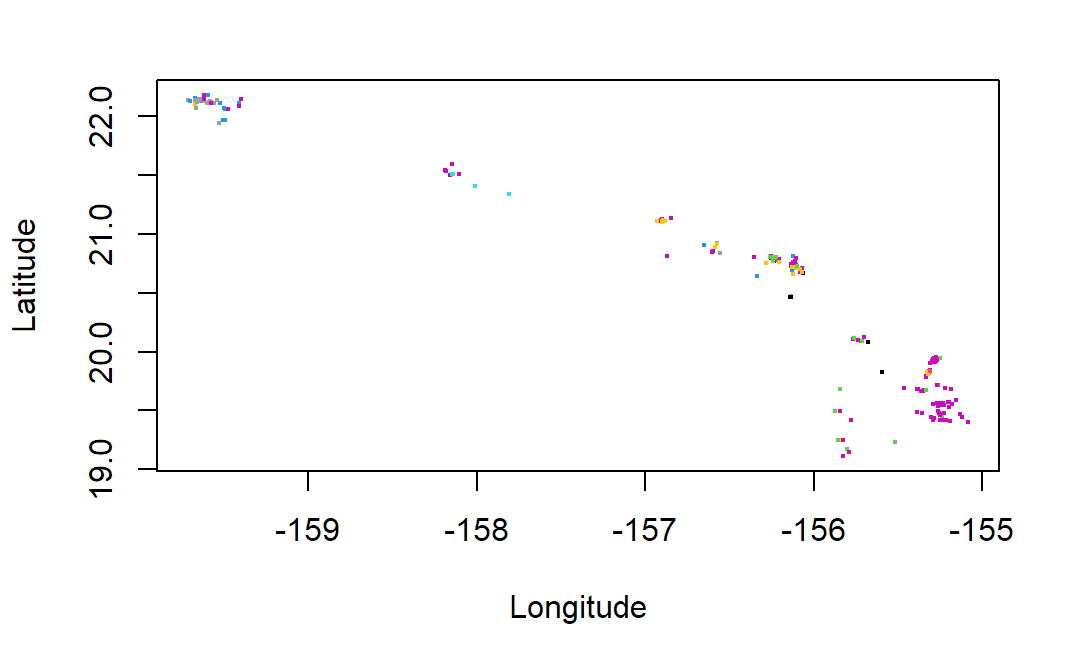
The occ() function returned an object of class occDat. It contains members for each database you could have queried, like “gbif” or “ebird”. Each of these members contains members called “data” which holds the actual data, and “meta” which contains metadata on what we searched for and how it was returned. The “data” object is a list where each member of the list holds a dataframe of records for a different species. As described we can use “bind_rows” from dplyr to create a composite dataframe from this list.
But wait, what is occurrence data?
Occurrence is related to abundance in that it also describes how species are distributed in space but is different in some important ways.
A single abundance data point describes the amount of individuals of a species in a certain area.
But a single occurrence data point describes the presence of a SINGLE individual in a location.
Occurrence data is vastly more common than abundance data online, but often comes with much greater bias in the way it captures the distribution of biodiversity. It is often “incidental”. A citizen scientist happening to record a new butterfly they saw on their morning hike (occurrence) or a researcher electing to record a rare beetle they were looking for (occurrence) are much less systematic and more biased than the field surveys specifically intended to monitor abundance.
Due to this bias it is often used just to indicate presence-absence of a species rather than the magnitude of its population size.
It can be possible to obtain “abundance-like” information from occurrences, but it requires VERY careful consideration of bias and uncertainty.
Phylogenetic trees from the Open Tree of Life
First we’ll get a clean list of taxonomic names from the GBIF
results. We could use our initial names we got from taxize,
but using our GBIF results conveniently narrows things down to Hawaii
species only.
R
species_names_hawaii <- unique(occurrences_df$name)
species_names_resolved <- gnr_resolve(species_names_hawaii, best_match_only = TRUE,
                          canonical = TRUE)
species_names_hawaii <- species_names_resolved$matched_name2
Now we can use the rotl package. The rotl
package provides an interface to the Open Tree of Life. To get a tree
from this database, we have to match our species names to OTOL’s
ids.
We first use trns_match_names() to match our species
names to OTOL’s taxonomy.
Then we use ott_id() to get OTOL ids for these matched
names.
R
species_names_otol <- tnrs_match_names(species_names_hawaii)
otol_ids <- ott_id(species_names_otol)
Finally, we get the tree containing these IDs as tips.
R
tr <- tol_induced_subtree(ott_ids = otol_ids)
plot(tr)
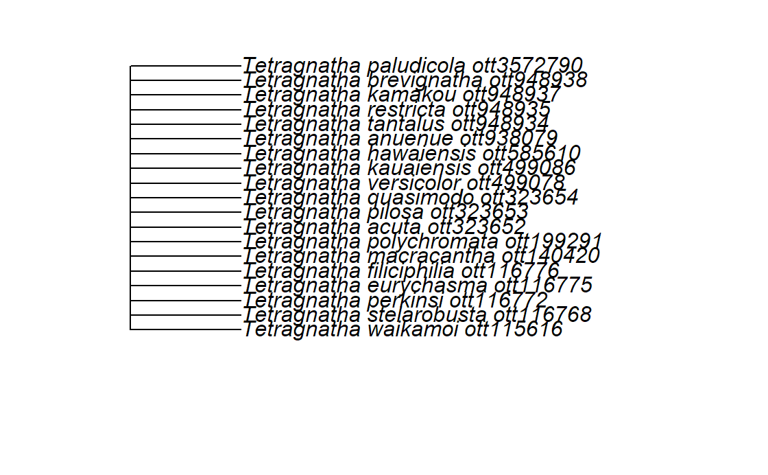
Unfortunately we can see that the phylogenetic relationships between these species aren’t resolved in OTOL, so we may have to look elsewhere for a phylogeny. This is an example of how not all the data we are looking for are in large repositories, especially higher resolution phylogenies.
Sequence data from NCBI
Let’s continue with the rentrez package, which provides
an interface to NCBI. The two usual steps for querying from NCBI is an
ID search using entrez_search() and a records fetch using those IDs in
entrez_fetch(). Sound a bit familiar?
We’ll again search for the species in our Hawaii occurrences.
The main arguments of the entrez_search() function are “db”, the database to look in, and “term” a string representing the whole query. While the occ() function had multiple fields for different ways we are narrowing our search, the “term” field wraps this up in a single string.
R
# we're using `species_names` that we made previously to make a long
# string of names that will be sent to NCBI via the ENTREZ API
termstring <- paste(sprintf('%s[ORGN]', species_names_hawaii), collapse = ' OR ')

search_results <- entrez_search(db="nucleotide", term = termstring)

# take a quick look at all the possible things we could have added to term for this database - it includes [GENE] for looking for specific genes or [SLEN] for length of sequence
entrez_db_searchable(db="nucleotide")
Unlike spocc but similarly to
rotl, this first search returns a set of IDs.
We then have to use entrez_fetch() on the IDs in
search_results to obtain the actual record information.
We specify ‘db’ as ‘nucleotide’ and ‘rettype’ as ‘fasta’ to get FASTA sequences
R
sequences <- entrez_fetch(db = "nucleotide", id = search_results$ids,
                          rettype = "fasta")

# just look at the first part of this *long* returned string
# substr gets characters 1 through 1148 of the FASTA, and cat simply prints it with line breaks
cat(substr(sequences,1,1148))
NCBI and OTOL both require an initial search to obtain record IDs, then a second fetch to obtain the actual record data for each ID
NCBI uses a string-based query where the search is a specially-formated string, while GBIF uses an argument-based query where the search is based on the various arguments you give to the R function.
NCBI is capable of taking a genus and returning the records of all its species, but OTOL and GBIF require obtaining the species names first using a package like taxize
GBIF data is formatted as a list of occurrences for each species contained in the object we get from the query.
Sources of MDBD: Databases without APIs
Many excellent databases exist without specialized APIs or R packages to facilitate their use.
For example, the BioTIME database is a compilation of timeseries of species ocurrence, abundance, and biomass data. It is openly available via the University of St. Andrews. The North American Breeding Bird Survey, run by the USGS, contains data on bird species abundances across the United States and Canada going back more than 50 years. These data are hosted on ScienceBase.
Some of these databases can be accessed via the Data Retriever and
accompanying R package the rdataretriever.
Some are findable via DataONE and the Ecological Data Initiative.
Others can be downloaded directly from the source.
Sources of MDBD: “small data” attached to papers
Finally, A lot of useful data is not held in databases, and is instead attached to papers. Searching manuscript databases or Google Scholar can be an effective way to find such data. You can filter Web of Science to find entries with “associated data”.
However, this can still be a somewhat heterogeneous and time-consuming strategy!
Recap
Keypoints
- Many sources exist online where multidimensional biodiversity data can be obtained
- APIs allow for fast and reproducible querying and downloading
- While there are patterns in how these APIs work, there will always be differences between databases that make using each API a bit different.
- Standalone databases and even the supplemental data in manuscripts can also be re-used.