Content from Introduction
Last updated on 2023-07-11 | Edit this page
Overview
Questions
- What do we mean by “multidimensional biodiversity data?
- What are the four types of data we’ll be covering in this workshop?
- What types of questions can we explore with these data?
- How will this workshop be structured? Where do I find course materials, etc?
Objectives
After following this episode, participants should be able to…
- Articulate a shared understanding of what “multidimensional biodiversity data” is
- List the types of data to be covered in this workshop, and potential applications of MBDB
- Locate course resources.
Welcome
Welcome everyone! This workshop will engage with ethics around biodiversity data through the lens of Indigenous data sovereignty and governance. With that in mind, many of the locations where this workshop might run will likely be unceded Indigenous lands. As part of our introductions we’ll think about where we are, where we come from, and our positionalities. Native Land Digital is a great resource for understanding where we are geographically, and here is a great video by Dr. Kat Gardner-Vandy and Daniella Scalice demonstrating classical academic introductions and relational introductions that center positionality:
Four dimensions of biodiversity data
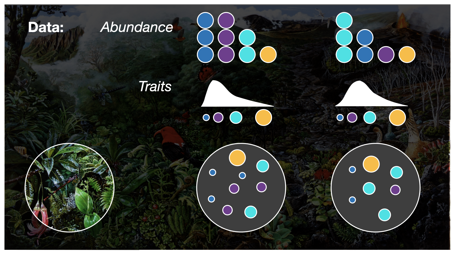
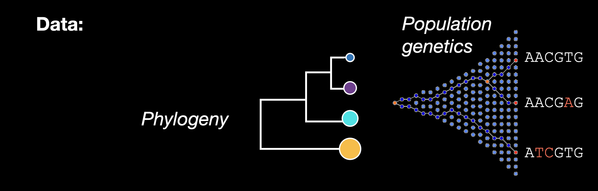
In this workshop, we’ll be working with four types of biodiversity data: species abundances, traits, population genetics, and phylogenetics. In this workshop, we’ll cover skills for working with each data type separately, and conclude with what we can accomplish when we integrate multiple data types into the same analysis.
To make this a little more interesting, we’ll ground our learning with a “real-world” (or, close to real-world) example!
For this workshop, we’ll be working with some simulated data based on real insect species found in the Hawaiian Islands The data contain real taxonomic names (so we can use workflows designed for dealing with real taxonomic data) but the abundances, traits, genetics, and phylogeny are simulated using a process model (more on that in Part II of this workshop).
Hawaiian sovereignty
Building from our acknowledgement of the Indigenous land where we gather for this workshop, we need to acknowledge that over a century of settler research has been conducted across the Hawaiian Islands without the consent of the Kanaka Maoli, the Native Hawaiians. The aina, or lands, of the Kanaka Maoli were stolen, their sovereignty illegally stripped, their culture, communities, and bodies killed. Sovereignty and the return of control of data to Indigenous people and communities is one of the learning objectives of this workshop. To start us on that journey, here are the words (watch on youtube) of Dr. Haunani-Kay Trask, a leader in the Hawaiian sovereignty movement:
We are not Americans! We will die as Hawaiians! We will never be Americans! I am here to explain what sovereignty is. Sovereignty, as many people say, is a feeling. The other day in the paper I read sovereignty is aloha, it’s love. Later on someone said it’s pride. No. Sovereignty is government. Sovereignty is government! It is an attribute of nationhood. We already have aloha. We already have pride. We already know who we are. Are we sovereign? No! Because we don’t have a government. Because we don’t control a land base. Sovereignty is not a feeling, it is the power of government. It is political power!

One of the contributions we as researchers can make to rematriation and repatriation of resources is to cede control of legacy biological data back to Indigenous communities, and preferably to engage in co-produced research from the beginning, where consent, governance, and mutual benefit are agreed upon before research begins. In Episode 3: CARE and FAIR principles, we will be learning about protocols developed by ENRICH and Local Contexts that center Indigenous data sovereignty and governance.
More about our simulated data
The Hawaiian Islands formed over a volcanic hotspot, as such Kauai is about 5 million years old, while the Big Island is still forming.
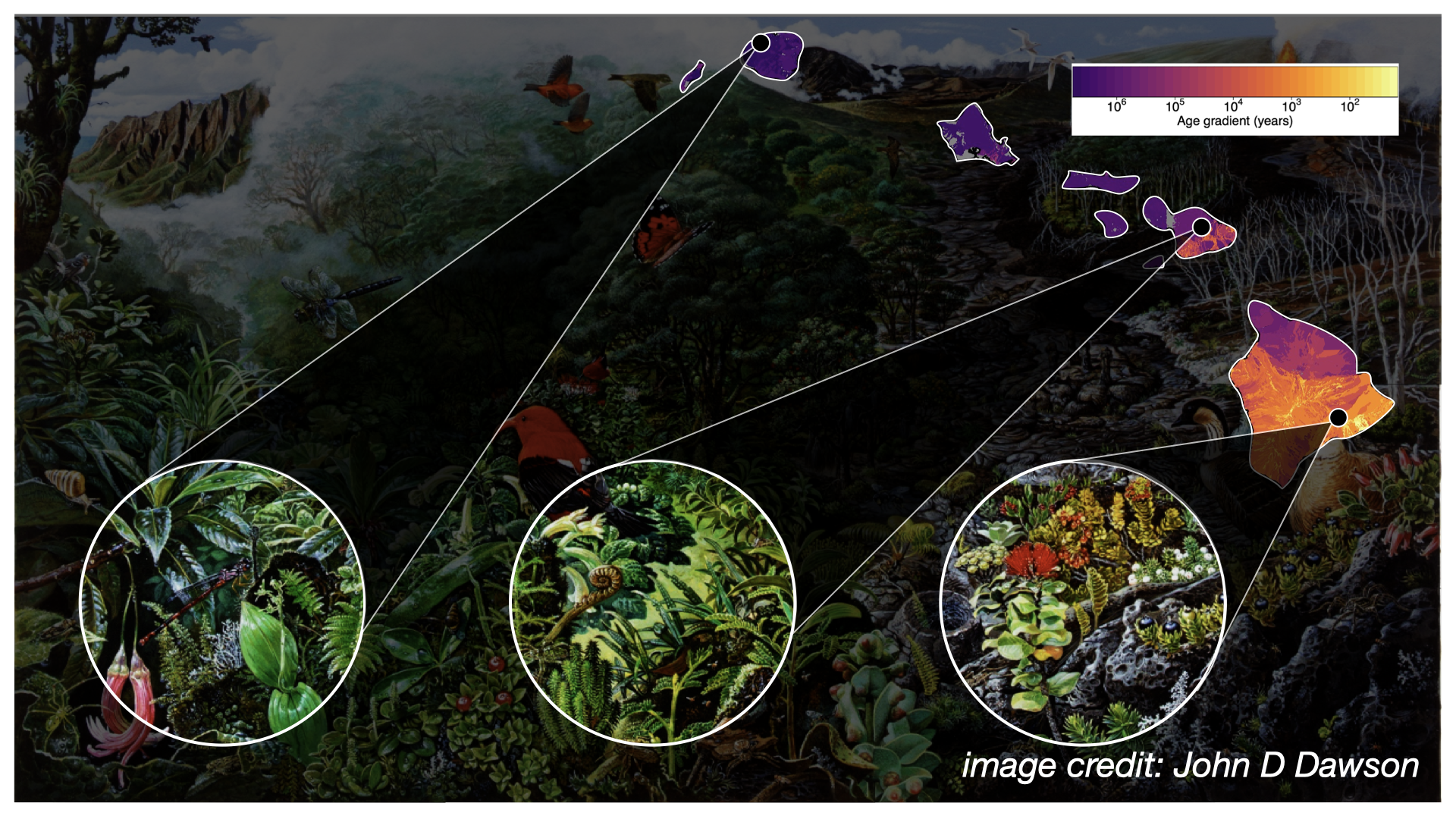
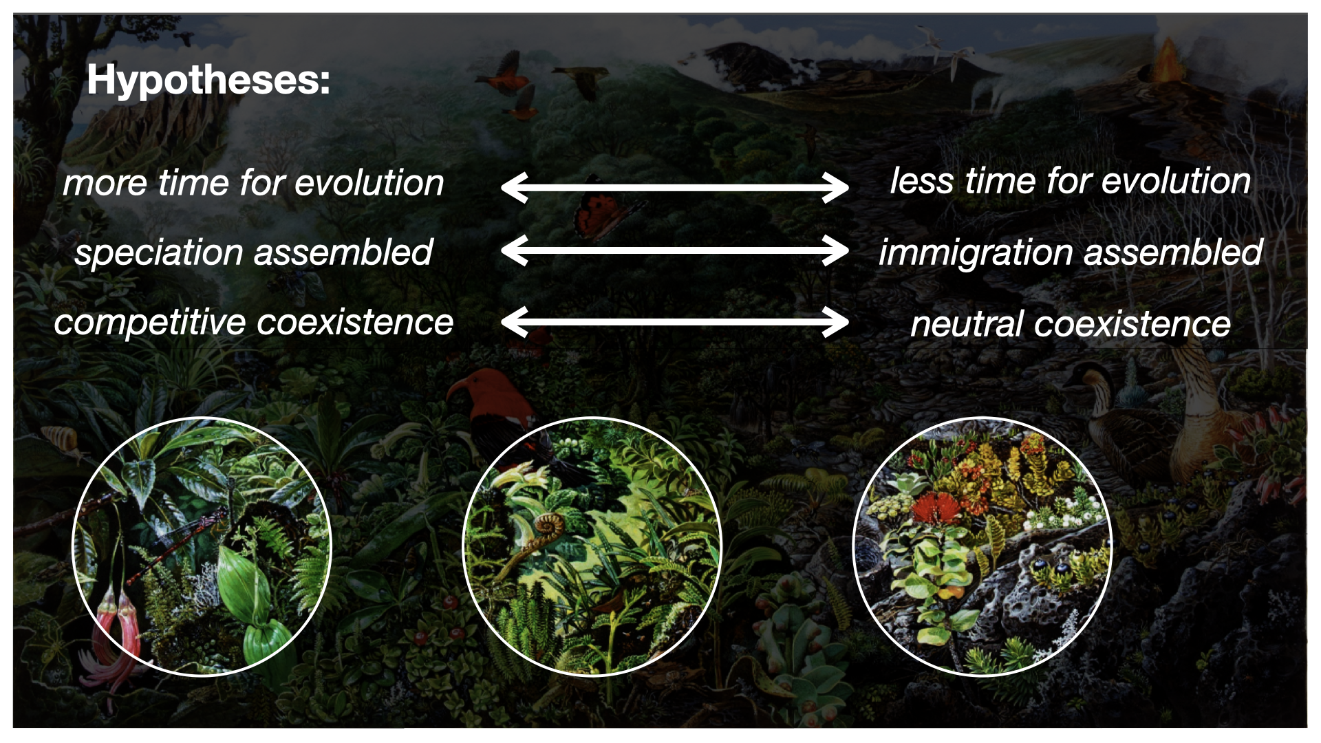
This chronosequence allows us to observe in the Modern (as opposed to the fossil record) what we might hypothesize to be different eco-evolutionary stages, or “snapshots,” of community assembly. We might further hypothesize that different assembly processes are more or less prevalent at different snapshots, such as increased importance of immigration early on, and greater importance of in situ diversification later on.
How are the four dimensions of biodiversity data conceptualized?
Workshop logistics and preview
For the rest of the workshop, we’ll take a tour of the data types and then bring them together.
Helpful links
Course website: https://role-model.github.io/multidim-biodiv-data/
Content from Indigenous Data Sovereignty and the CARE Principles
Last updated on 2023-07-11 | Edit this page
Overview
Questions
- What is Indigenous data sovereignty?
- What are the CARE principles?
- What is Local Contexts Hub, and how can we use it to implement the CARE principles in our work?
Objectives
After following this episode, we intend that participants will be able to:
- Articulate the mission of Local Contexts in the context of the CARE and FAIR principles
- Create an account on Local Contexts Hub
- Create a project on Local Contexts Hub
- Apply Bio-Cultural and Traditional Knowledge Notices appropriately to datasets
Indigenous data soverginty
To aid in our learning about and discussion of Indigenous data soverginty we will watch this video from Local Contexts:
The CARE Principles
The CARE principles developed by Stephanie Russo Carroll et al. codify Indigenous data sovereignty into actionable standards for data governance. The CARE principles are designed to live alongside and make more just the FAIR principles. The FAIR principles are seen as also being a necessary of Indigenous data sovereignty and governance
Collective benefit
Collective benefit means that the communities from which data are gathered should share in any benefit derived from those data.
Authority to control
Authority to control means that communities have the right and authority to govern how data pertaining to themselves (their cultures, knowledges, bodies, environments) is gathered, used, shared, and re-used.
Implementing the CARE Principles through the Local Contexts Hub
Local Contexts Hub serves Traditional Knowledge Labels and Notices, and Biocultural Labels and Notices. We learned about those in the video from Local Contexts, now we’ll learn how Labels and Notices can operationalize the CARE principles.
Follow along with this slide deck.
Challenge
Set up your own account on Local Contexts Hub!
Keypoints
- “Be FAIR and CARE”: The CARE principles (Collective benefit, Authority to control, Responsibility, and Ethics) are part of a framework emphasizing Indigenous rights and interests in the context of data sharing ecosystems.
- Local Contexts Hub provides Labels and Notices for learning more about and engaging with Indigenous data in accordance with the CARE principles.
- Work remains to be done in order to spread the use of TK and BC Labels/Notices by researchers and data repositories
Content from Abundance Data
Last updated on 2023-07-11 | Edit this page
Overview
Questions
- What is abundance data, and how can we use it to gain insights about a system?
- How do I clean and manipulate abundance data to prepare for analyses?
- How do I calculate summary statistics and relate these to ecological pattern?
Objectives
After following this episode, participants should be able to…
- Describe ecological abundance data and what it can tell us about a system
- Import and examine organismal abundance data from .csv files
- Clean taxonomic names
- Manipulate abundance data into different formats
- Generate species abundance distribution plots from abundance data
- Summarize species abundance data using Hill numbers
- Interpret how different Hill numbers correspond to different signatures of species diversity
Introduction to abundance data
Abundance data is one of the most widely-collected biodiversity data types. It generally keeps track of how many individuals of each species (or taxonomic unit) are present at a site. It may also be recorded as relative abundances or percent cover, depending on the group.
There’s a huge diversity of applications of abundance data. Here, we’ll focus on one of the most generally-applicable approaches, which is to look at the diversity of a system. By diversity, we mean how abundance is distributed among the different taxonomic groups present in that system. This incorporates both species richness, and the evenness of how abundances is portioned among different species.
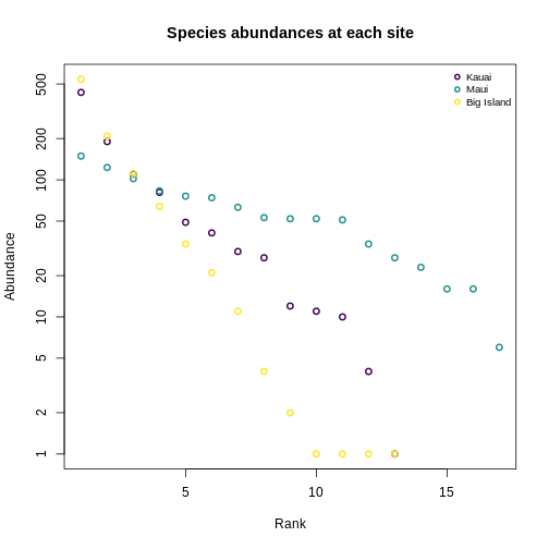
Let’s make this more concrete. If we plot the abundances of all the species in a system, sorted from most to least abundant, we end up with something like this:
This is the species abundance distribution, or SAD.
The SAD can show how even or uneven our system is.
Ok, great. What if we want to make comparisons between different systems? For that we need a quantifiable metric.
There are dozens - literally - of summary statistics for ecological diversity.
For this workshop, we’re going to focus on Hill numbers.
Hill numbers are a family of diversity indices that can be described verbally as the “effective number of species”. That is, they describe how many species of equal abundances would be present in a system to generate the corresponding diversity index.
Hill numbers are similar to other diversity indices you might have encountered. In fact, they mathematically converge with Shannon, Simpson, and species evenness.
Working with abundance data
Ok, so how about we do some actual coding?
For this episode, we’ll be working with a couple of specialized packages for biological data.
R
library(dplyr)
library(taxize)
library(hillR)
library(vegan)
library(tidyr)
Loading data
We’ll be working with ecological species abundance data stored in
.csv files. For help working with other storage formats, the
Carpentries’ Ecological Data lesson materials on databases are a
great place to start!
Let’s load the data:
R
abundances <- read.csv("https://raw.githubusercontent.com/role-model/multidim-biodiv-data/main/episodes/data/abundances_raw.csv")
And look at what we’ve got:
R
head(abundances)
OUTPUT
     island  site                GenSp abundance
1 BigIsland BI_01         Cis signatus       541
2 BigIsland BI_01 Acanthia procellaris        64
3 BigIsland BI_01     Spoles solitaria        34
4 BigIsland BI_01        Laupala pruna        21
5 BigIsland BI_01  Toxeuma hawaiiensis       111
6 BigIsland BI_01  Chrysotus parthenus       208
abundances is a data frame with columns for
island, site, GenSp, and
abundance. Each row tells us how many individuals of each
species (GenSp) were recorded at a given site on each island. This is a
common format - imagine you are censusing a plant quadrat, counting up
how many individuals of each species you see.
Cleaning taxonomic names
The first thing we’ll want to do is check for human error wherever we can, in this case in the form of typos in data entry.
The taxize R package can help identify and resolve
simple typos in taxonomic names.
R
species_list <- abundances$GenSp

name_resolve <- gnr_resolve(species_list, best_match_only = TRUE,
                            canonical = TRUE) # returns only name, not authority
R
head(name_resolve)
OUTPUT
# A tibble: 6 × 5
  user_supplied_name   submitted_name      data_source_title score matched_name2
  <chr>                <chr>               <chr>             <dbl> <chr>
1 Cis signatus         Cis signatus        Encyclopedia of … 0.988 Cis signatus
2 Acanthia procellaris Acanthia procellar… uBio NameBank     0.988 Acanthia pro…
3 Spoles solitaria     Spoles solitaria    Catalogue of Lif… 0.75  Spolas solit…
4 Laupala pruna        Laupala pruna       National Center … 0.988 Laupala pruna
5 Toxeuma hawaiiensis  Toxeuma hawaiiensis Encyclopedia of … 0.988 Toxeuma hawa…
6 Chrysotus parthenus  Chrysotus parthenus Encyclopedia of … 0.988 Chrysotus pa…
R
mismatches <- name_resolve[ name_resolve$matched_name2 !=
                                name_resolve$user_supplied_name, ]

mismatches[, c("user_supplied_name", "matched_name2")]
OUTPUT
# A tibble: 6 × 2
  user_supplied_name       matched_name2
  <chr>                    <chr>
1 Spoles solitaria         Spolas solitaria
2 Metrothorax deverilli    Metrothorax
3 Agonosmus argentiferus   Agonismus argentiferus
4 Agrotis chersotoides     Agrotis
5 Proterhenus punctipennis Proterhinus punctipennis
6 Elmoea lanceolata        Elmoia lanceolata
Four of these are just typos. But Agrotis chersotoides
in our data is resolved only to Agrotis and
Metrothorax deverilli is resolved to
Metrothorax. What’s up there?
R
name_resolve$matched_name2[
    name_resolve$user_supplied_name == "Agrotis chersotoides"] <-
    "Peridroma chersotoides"

name_resolve$matched_name2[
    name_resolve$user_supplied_name == "Metrothorax deverilli"] <-
    "Metrothorax deverilli"
Now we need to add the newly-resolved names to our
abundances data. For this, we’ll use a function called
left_join.
R
abundances <- left_join(abundances, name_resolve, by = c("GenSp" = "user_supplied_name"))

abundances$final_name <- abundances$matched_name2

head(abundances)
OUTPUT
     island  site                GenSp abundance       submitted_name
1 BigIsland BI_01         Cis signatus       541         Cis signatus
2 BigIsland BI_01 Acanthia procellaris        64 Acanthia procellaris
3 BigIsland BI_01     Spoles solitaria        34     Spoles solitaria
4 BigIsland BI_01        Laupala pruna        21        Laupala pruna
5 BigIsland BI_01  Toxeuma hawaiiensis       111  Toxeuma hawaiiensis
6 BigIsland BI_01  Chrysotus parthenus       208  Chrysotus parthenus
                              data_source_title score        matched_name2
1                          Encyclopedia of Life 0.988         Cis signatus
2                                 uBio NameBank 0.988 Acanthia procellaris
3                   Catalogue of Life Checklist 0.750     Spolas solitaria
4 National Center for Biotechnology Information 0.988        Laupala pruna
5                          Encyclopedia of Life 0.988  Toxeuma hawaiiensis
6                          Encyclopedia of Life 0.988  Chrysotus parthenus
            final_name
1         Cis signatus
2 Acanthia procellaris
3     Spolas solitaria
4        Laupala pruna
5  Toxeuma hawaiiensis
6  Chrysotus parthenus
Visualizing species abundance distributions
Now that we have cleaned data, we can generate plots of how abundance is distributed.
Because we’ll want to look at each island separately, we’ll use the
split command to break the abundances data
frame apart by island. split will split a dataframe into
groups defined by the f argument (for “factor”) - in this
case, the different values of the island column of the
abundances data frame:
R
island_abundances <- split(abundances, f = abundances$island)
Usual practice is to plot distributions of abundance as the species abundance on the y-axis and the rank of that species (from most-to-least-abundant) on the x-axis. This allows us to make comparisons between sites that don’t have any species in common.
Now, we’ll construct a plot with lines for the abundances of species on each island.
R
# figure out max number of species at a site for axis limit setting below
max_sp <- sapply(island_abundances, nrow)
max_sp <- max(max_sp)

plot(
    sort(island_abundances$Kauai$abundance, decreasing = TRUE),
    main = "Species abundances at each site",
    xlab = "Rank",
    ylab = "Abundance",
    lwd = 2,
    col = "#440154FF",
    xlim = c(1, max_sp),
    ylim = c(1, max(abundances$abundance)),
    log = 'y'
)

points(
    sort(island_abundances$Maui$abundance, decreasing = T),
    lwd = 2,
    col = "#21908CFF"
)

points(
    sort(island_abundances$BigIsland$abundance, decreasing = T),
    lwd = 2,
    col = "#FDE725FF"
)

legend(
    "topright",
    legend = c("Kauai", "Maui", "Big Island"),
    pch = 1,
    pt.lwd = 2,
    col = c("#440154FF", "#21908CFF", "#FDE725FF"),
    bty = "n",
    cex = 0.8
)

Quantifying diversity using Hill numbers
Let’s calculate Hill numbers to put some numbers to these shapes.
For this, we’ll need what’s known as a site by species matrix. This is a very common data format for ecological diversity data.
Site-by-species matrix
A site by species sites as rows and species as columns. We can get
there using the pivot_wider function from the package
tidyr:
R
abundances_wide <- pivot_wider(abundances, id_cols = site,
                              names_from = final_name,
                              values_from = abundance,
                              values_fill = 0)

head(abundances_wide[,1:10])
OUTPUT
# A tibble: 3 × 10
  site  `Cis signatus` `Acanthia procellaris` `Spolas solitaria` `Laupala pruna`
  <chr>          <int>                  <int>              <int>           <int>
1 BI_01            541                     64                 34              21
2 MA_01             52                     53                  0               0
3 KA_01              0                      0                  0              12
# ℹ 5 more variables: `Toxeuma hawaiiensis` <int>, `Chrysotus parthenus` <int>,
#   `Metrothorax deverilli` <int>, `Drosophila obscuricornis` <int>,
#   `Cis bimaculatus` <int>
We’ll want this data to have row names based on the sites, so we’ll need some more steps:
R
abundances_wide <- as.data.frame(abundances_wide)

row.names(abundances_wide) <- abundances_wide$site

abundances_wide <- abundances_wide[, -1]

head(abundances_wide)
OUTPUT
      Cis signatus Acanthia procellaris Spolas solitaria Laupala pruna
BI_01          541                   64               34            21
MA_01           52                   53                0             0
KA_01            0                    0                0            12
      Toxeuma hawaiiensis Chrysotus parthenus Metrothorax deverilli
BI_01                 111                 208                    11
MA_01                 102                  27                     0
KA_01                   0                   0                   190
      Drosophila obscuricornis Cis bimaculatus Nysius lichenicola
BI_01                        2               4                  1
MA_01                       83             149                 16
KA_01                        0               0                  0
      Agonismus argentiferus Peridroma chersotoides Scaptomyza villosa
BI_01                      1                      1                  1
MA_01                      0                     23                 63
KA_01                      0                      0                  0
      Lispocephala dentata Hylaeus facilis Laupala vespertina
BI_01                    0               0                  0
MA_01                  123              74                 52
KA_01                    0               0                  0
      Proterhinus punctipennis Nesomicromus haleakalae Odynerus erythrostactes
BI_01                        0                       0                       0
MA_01                       51                      76                      34
KA_01                      434                       0                       0
      Eurynogaster vittata Elmoia lanceolata Xyletobius collingei
BI_01                    0                 0                    0
MA_01                    6                16                    0
KA_01                    0                 0                   41
      Nesodynerus mimus Scaptomyza vagabunda Lucilia graphita
BI_01                 0                    0                0
MA_01                 0                    0                0
KA_01                30                   81               49
      Eudonia lycopodiae Atelothrus depressus Mecyclothorax longulus
BI_01                  0                    0                      0
MA_01                  0                    0                      0
KA_01                110                   10                     11
      Hylaeus sphecodoides Hyposmocoma sagittata Campsicnemus nigricollis
BI_01                    0                     0                        0
MA_01                    0                     0                        0
KA_01                    4                    27                        1
Let’s write it to a file in case we need to load it again later on:
R
write.csv(abundances_wide, here::here("episodes", "data", "abundances_wide.csv"), row.names = F)
WARNING
Warning in file(file, ifelse(append, "a", "w")): cannot open file
'/home/runner/work/multidim-biodiv-data/multidim-biodiv-data/site/built/episodes/data/abundances_wide.csv':
No such file or directory
ERROR
Error in file(file, ifelse(append, "a", "w")): cannot open the connectionCalculating Hill numbers with hillR
The hillR package allows us to calculate Hill
numbers.
R
hill_0 <- hill_taxa(abundances_wide, q = 0)

hill_0
OUTPUT
BI_01 MA_01 KA_01
   13    17    13
R
hill_1 <- hill_taxa(abundances_wide, q = 1)

hill_1
OUTPUT
    BI_01     MA_01     KA_01
4.001789 13.746057 5.949875 R
hill_2 <- hill_taxa(abundances_wide, q = 2)

hill_2
OUTPUT
    BI_01     MA_01     KA_01
 2.824029 11.958289  4.012680
Relating Hill numbers to patterns in diversity
Let’s revisit the SAD plots we generated before, and think about these in terms of Hill numbers.
R
plot(
    sort(island_abundances$Kauai$abundance, decreasing = TRUE),
    main = "Species abundances at each site",
    xlab = "Rank",
    ylab = "Abundance",
    lwd = 2,
    col = "#440154FF",
    xlim = c(1, max_sp),
    ylim = c(1, max(abundances$abundance)),
    log = 'y'
)

points(
    sort(island_abundances$Maui$abundance, decreasing = T),
    lwd = 2,
    col = "#21908CFF"
)

points(
    sort(island_abundances$BigIsland$abundance, decreasing = T),
    lwd = 2,
    col = "#FDE725FF"
)

legend(
    "topright",
    legend = c("Kauai", "Maui", "Big Island"),
    pch = 1,
    pt.lwd = 2,
    col = c("#440154FF", "#21908CFF", "#FDE725FF"),
    bty = "n",
    cex = 0.8
)
R
hill_abund <- data.frame(hill_abund_0 = hill_0,
                         hill_abund_1 = hill_1,
                         hill_abund_2 = hill_2)
hill_abund <- cbind(site = rownames(hill_abund), hill_abund)

rownames(hill_abund) <- NULL

hill_abund
OUTPUT
   site hill_abund_0 hill_abund_1 hill_abund_2
1 BI_01           13     4.001789     2.824029
2 MA_01           17    13.746057    11.958289
3 KA_01           13     5.949875     4.012680
Recap
Keypoints
- Organismal abundance data are a fundamental data type for population and community ecology.
- The
taxisepackage can help with data cleaning, but quality checks are often ultimately dataset-specific. - The species abundance distribution (SAD) summarizes site-specific abundance information to facilitate cross-site or over-time comparisons.
- We can quantify the shape of the SAD using summary statistics. Specifically, Hill numbers provide a unified framework for describing the diversity of a system.
Content from Trait data
Last updated on 2023-07-11 | Edit this page
Overview
Questions
- What information is captured via trait data?
- How do you read, clean, and visualize trait data?
- What do Hill numbers convey in the context of trait data?
Objectives
After following this episode, participants should be able to…
- Import trait data in a CSV format into the R environment
- Clean taxonomic names using the
taxizepackage - Aggregate traits
- Visualize trait distributions
- Calculate Hill numbers
- Interpret Hill numbers using ranked trait plots
Introduction to traits
Trait data is both old and new in ecology.
Similarly to abundance, investigating trait data can give insights into the ecological processes shaping different communities. Specifically, it would be interesting to answer questions like: 1) how much does a specific trait vary in a community?; 2) Are all species converging into a similar trait value or dispersing into a wide range of values for the trait?; 3) do those patterns of variation change across different communities? Answering these questions can help us understand how species are interacting with the environment and/or with each other.
Defining what exactly constitutes a trait, and measuring traits, can get complicated in ecology. (For example, there are lots of things we can measure about even just a leaf - but it’s another story to understand which of those attributes are telling us something ecologically meaningful). Ideally, we’d want to focus on a trait that is easily measurable and also linked to ecological features of interest. One such trait is body size. Body size is correlated with a whole host of ecologically meaningful traits, and is one of the easiest things to measure about an organism.
Similarly to how we look at community-wide distributions of abundance, we can generate and interpret community-wide trait distributions.
And, similar to how we can look at species abundance diversity using Hill numbers, we can look at trait diversity using a trait Hill number.
Working with trait data
Importing and cleaning trait data
Here, we will work with a dataset containing values of body mass for the species in the Hawaiian islands. Unlike the abundance data, each row represents one specimen: in this dataset, each row contains the body mass measured for that specimen. Our overall goal here is to clean this data and attach it to the species data, so we can investigate trait patterns per community.
We’re starting with a challenge! First, let’s load the packages we’ll need for the whole episode (you won’t need all of them for this first challenge)
R
library(taxize)
library(dplyr)
OUTPUT
Attaching package: 'dplyr'OUTPUT
The following objects are masked from 'package:stats':

    filter, lag
OUTPUT
The following objects are masked from 'package:base':

    intersect, setdiff, setequal, union
R
library(tidyr)
library(hillR)
Challenge
In the abundance-data episode, you learned how to read in a
CSV file with the read.csv() function. In
addition, you learned how to clean and standardize the taxonomic
information in your data set using the gnr_resolve()
function from the taxize package.
You’re going to use those skills to import and clean the trait data
set. The trait data set contains two columns: GenSp, which
contains the binomial species names, and mass_g, which
contains the individual’s mass in grams, the metric of body size chosen
for the study. The data also contain typos and a problem with the
taxonomy that you must correct and investigate. Make sure to glance at
the data before cleaning!
Your trait data is located at: https://raw.githubusercontent.com/role-model/multidim-biodiv-data/main/episodes/data/body_size_data.csv
Read in the traits data using the read.csv function and
supplying it with the path to the data.
R
traits <- read.csv('https://raw.githubusercontent.com/role-model/multidim-biodiv-data/main/episodes/data/body_size_data.csv')

head(traits)
OUTPUT
         GenSp   mass_g
1 Cis signatus 2.499395
2 Cis signatus 2.544560
3 Cis signatus 3.045801
4 Cis signatus 2.471702
5 Cis signatus 3.427594
6 Cis signatus 2.520676
Check the names of the traits using the gnr_resolve()
function. To streamline your efforts, supply only the unique species
names in your data to gnr_resolve().
R
# only need to check the unique names
species_list <- unique(traits$GenSp)

name_resolve <- gnr_resolve(species_list, best_match_only = TRUE,
                            canonical = TRUE)

head(name_resolve)
OUTPUT
# A tibble: 6 × 5
  user_supplied_name   submitted_name      data_source_title score matched_name2
  <chr>                <chr>               <chr>             <dbl> <chr>
1 Cis signatus         Cis signatus        Encyclopedia of … 0.988 Cis signatus
2 Acanthia procellaris Acanthia procellar… uBio NameBank     0.988 Acanthia pro…
3 Spolas solitaria     Spolas solitaria    Encyclopedia of … 0.988 Spolas solit…
4 Spolas solitari      Spolas solitari     Catalogue of Lif… 0.75  Spolas solit…
5 Laupala pruna        Laupala pruna       National Center … 0.988 Laupala pruna
6 Toxeuma hawaiiensis  Toxeuma hawaiiensis Encyclopedia of … 0.988 Toxeuma hawa…
To quickly see which taxa are in conflict with taxize’s,
use bracket subsetting and Boolean matching.
R
mismatches_traits <-
    name_resolve[name_resolve$user_supplied_name != name_resolve$matched_name2,
                 c("user_supplied_name", "matched_name2")]

mismatches_traits
OUTPUT
# A tibble: 10 × 2
   user_supplied_name      matched_name2
   <chr>                   <chr>
 1 Spolas solitari         Spolas solitaria
 2 Metrothorax deverilli   Metrothorax
 3 Drosophila obscuricorni Drosophila obscuricornis
 4 Cis bimaculatu          Cis bimaculatus
 5 Agrotis chersotoides    Agrotis
 6 Eurynogaster vittat     Eurynogaster vittata
 7 Atelothrus depressu     Atelothrus depressus
 8 Hylaeus sphecodoide     Hylaeus sphecodoides
 9 Hyposmocoma sagittat    Hyposmocoma sagittata
10 Campsicnemus nigricolli Campsicnemus nigricollis
Fixing the names comes in two steps. First, we join the
traits dataframe with the name_resolve
dataframe using the left_join() function. Note, we indicate
that the GenSp and user_supplied_name columns
have the same information by supplying a named vector to the
by = argument.
R
traits <- left_join(traits,
                    name_resolve[, c("user_supplied_name", "matched_name2")],
                    by = c("GenSp" = "user_supplied_name"))

head(traits)
OUTPUT
         GenSp   mass_g matched_name2
1 Cis signatus 2.499395  Cis signatus
2 Cis signatus 2.544560  Cis signatus
3 Cis signatus 3.045801  Cis signatus
4 Cis signatus 2.471702  Cis signatus
5 Cis signatus 3.427594  Cis signatus
6 Cis signatus 2.520676  Cis signatus
Then, to fix Agrotis chersotoides and Metrothorax deverilli, as in abundance-data episode, use bracketed indexing, boolean matching, and assignment.
In addition, although not necessary, changing the column name
matched_name2 to final_name to give it a more
sensible name for later use is good practice.
R
traits$matched_name2[traits$matched_name2 == "Agrotis"] <-
    "Peridroma chersotoides"

traits$matched_name2[traits$matched_name2 == "Metrothorax"] <-
    "Metrothorax deverilli"

colnames(traits)[colnames(traits) == "matched_name2"] <- "final_name"

head(traits)
OUTPUT
         GenSp   mass_g   final_name
1 Cis signatus 2.499395 Cis signatus
2 Cis signatus 2.544560 Cis signatus
3 Cis signatus 3.045801 Cis signatus
4 Cis signatus 2.471702 Cis signatus
5 Cis signatus 3.427594 Cis signatus
6 Cis signatus 2.520676 Cis signatus
Summarizing and cleaning trait data
When analyzing trait data, it often needs to be summarized at a higher level than the individual. For instance, many community assembly analyses require species-level summaries, rather than individual measurements. So, we often want to calculate summary statistics of traits for each species. For numeric measurements, body size, statistics like the mean, median, and standard deviation give information about the center and spread of the distribution of traits for the species. For this section, you will aggregate the trait data to the species level, calculating the mean, median, and mode of body size for each species.
While there are methods to aggregate data in base R, the dplyr makes this task and other
data wrangling tasks much more intuitive. The function
group_by() groups your data frame by a variable. The first
argument to group_by() is your data frame, and all
following unnamed arguments are the variables you want to group the data
by. In our case, we want to group by species name, so we’ll supply
final_name.
R
library(dplyr)

# group the data frame by species
traits_sumstats <- group_by(traits, final_name)
group_by() just adds an index that tells any following
dplyr functions to perform their calculations on the group
the data frame was indexed by. So, to perform the actual calculations,
we will use the summarize() function
(summarise() works too for non-Americans). The first
argument you supply is the data frame, following by the calculations you
want to perform on the grouped data and what you want to name the
resulting variables. The structure is
new_var_name = function(original_var_name) for each
calculation. Here, we’re using the mean(),
median(), and sd() functions. Then, we’ll take
a look at the new data set with the head() function.
R
# summarize the grouped data frame, so you're calculating the summary statistics for each species
traits_sumstats <-
    summarize(
        traits_sumstats,
        mean_mass_g = mean(mass_g),
        median_mass_g = median(mass_g),
        sd_mass_g = sd(mass_g)
    )

head(traits_sumstats)
OUTPUT
# A tibble: 6 × 4
  final_name               mean_mass_g median_mass_g sd_mass_g
  <chr>                          <dbl>         <dbl>     <dbl>
1 Acanthia procellaris           1.09          1.13     0.241
2 Agonismus argentiferus         5.31          5.55     0.992
3 Atelothrus depressus           0.529         0.521    0.127
4 Campsicnemus nigricollis       0.422         0.375    0.0992
5 Chrysotus parthenus            1.77          1.70     0.273
6 Cis bimaculatus                2.31          2.27     0.605
Finally, you need to add the aggregated species-level information back to the abundance data, so you have the summary statistics for each species at each site.
First, re-read in the abundance data you used in the abundance episode.
R
abundances <- read.csv("https://raw.githubusercontent.com/role-model/multidim-biodiv-data/main/episodes/data/abundances_resolved.csv")

head(abundances)
OUTPUT
     island  site                GenSp abundance       submitted_name
1 BigIsland BI_01         Cis signatus       541         Cis signatus
2 BigIsland BI_01 Acanthia procellaris        64 Acanthia procellaris
3 BigIsland BI_01     Spoles solitaria        34     Spoles solitaria
4 BigIsland BI_01        Laupala pruna        21        Laupala pruna
5 BigIsland BI_01  Toxeuma hawaiiensis       111  Toxeuma hawaiiensis
6 BigIsland BI_01  Chrysotus parthenus       208  Chrysotus parthenus
                              data_source_title score        matched_name2
1                          Encyclopedia of Life 0.988         Cis signatus
2                                 uBio NameBank 0.988 Acanthia procellaris
3                   Catalogue of Life Checklist 0.750     Spolas solitaria
4 National Center for Biotechnology Information 0.988        Laupala pruna
5                          Encyclopedia of Life 0.988  Toxeuma hawaiiensis
6                          Encyclopedia of Life 0.988  Chrysotus parthenus
            final_name
1         Cis signatus
2 Acanthia procellaris
3     Spolas solitaria
4        Laupala pruna
5  Toxeuma hawaiiensis
6  Chrysotus parthenus
To join the data, you’ll use left_join(), which is
hopefully getting familiar to you now!
abundances should be on the left side, since we want the
species-information for each species in each community.
R
traits_sumstats <- left_join(abundances,
                             traits_sumstats,
                             by = "final_name")

head(traits_sumstats)
OUTPUT
     island  site                GenSp abundance       submitted_name
1 BigIsland BI_01         Cis signatus       541         Cis signatus
2 BigIsland BI_01 Acanthia procellaris        64 Acanthia procellaris
3 BigIsland BI_01     Spoles solitaria        34     Spoles solitaria
4 BigIsland BI_01        Laupala pruna        21        Laupala pruna
5 BigIsland BI_01  Toxeuma hawaiiensis       111  Toxeuma hawaiiensis
6 BigIsland BI_01  Chrysotus parthenus       208  Chrysotus parthenus
                              data_source_title score        matched_name2
1                          Encyclopedia of Life 0.988         Cis signatus
2                                 uBio NameBank 0.988 Acanthia procellaris
3                   Catalogue of Life Checklist 0.750     Spolas solitaria
4 National Center for Biotechnology Information 0.988        Laupala pruna
5                          Encyclopedia of Life 0.988  Toxeuma hawaiiensis
6                          Encyclopedia of Life 0.988  Chrysotus parthenus
            final_name mean_mass_g median_mass_g   sd_mass_g
1         Cis signatus  2.75162128    2.53261792 0.395389440
2 Acanthia procellaris  1.09171586    1.13005561 0.241013781
3     Spolas solitaria  3.01819088    3.19822329 0.612003059
4        Laupala pruna  0.05259815    0.05058839 0.009513021
5  Toxeuma hawaiiensis  2.16818518    2.20868688 0.301463517
6  Chrysotus parthenus  1.76717404    1.69687138 0.273022541
Visualizing trait distributions
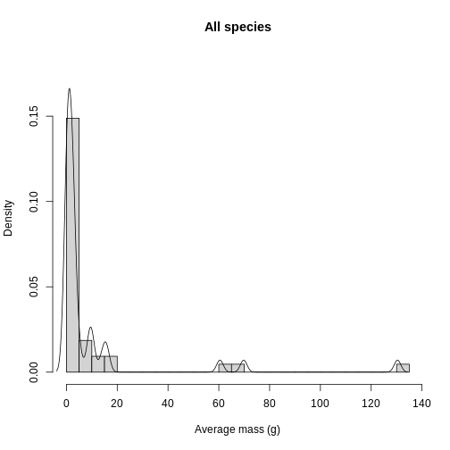
Histograms and density plots can help give you a quick look at the distribution of your data. For quality control purposes, they are useful to see if there are any suspicious values due to human error. Let’s overlay the histogram and density plots to get an idea of what aggregated (histogram) and smoothed (density) representations of the data look like.
The first argument to the hist() function is your data.
breaks sets the number of histogram bars, which can be
tuned heuristically to find a number of bars that best represents the
distribution of your data. I found that breaks = 40 is a
reasonable value. xlab, ylab, and
main are all used to specify labels for the x-axis, y-axis,
and title, respectively. When scaling the plot, sometimes base R
plotting functions aren’t as responsive to the data as we like. To fix
this, you can use the xlim or ylim functions
to set the value range of the x-axis and y-axis, respectively. Here, we
set ylim to a vector c(0, 0.11), which
specifies the y-axis to range from 0 to 0.11.
If you’re used to seeing histograms, the y-axis may look unfamiliar.
To get the two plots to use the same scale, you set
freq = FALSE, which converts the histogram counts to a
density value. The density scales the distribution from 0-1, so the bar
height (and line height on the density plot) is a fraction of the total
distribution.
Finally, to add the density line to the plot, you calculate the
density of the trait distribution with the density()
function and wrap it with the lines() function.
R
hist(
    traits_sumstats$mean_mass_g,
    breaks = 40,
    xlab = "Average mass (g)",
    ylab = "Density",
    main = "All species",
    ylim = c(0,0.18),
    freq = FALSE
)

lines(density(traits_sumstats$mean_mass_g))
In addition to quality control, knowing the distribution of trait data lends itself towards questions of what processes are shaping the communities under study. Are the traits overdispersed? Underdispersed? Does the average vary across communities? To get at these questions, you need to plot each site and compare among sites. To facilitate comparison, you’re going to layer the distributions on top of each other in a single plot. Histograms get cluttered quickly, so let’s use density plots for this task.
To plot each site, you need a separate dataframe for each site. The
easiest way to do this is with the split() function, which
takes a dataframe followed by a variable to split the dataframe by. It
then returns a list of data frames for each element in the variable.
Running head() on the list returns a lot of output, so
you can use the names() function to make sure the names of
the dataframes in your list are the sites you intended to split by.
R
# split by site
traits_sumstats_split <- split(traits_sumstats, traits_sumstats$site)

names(traits_sumstats_split)
OUTPUT
[1] "BI_01" "KA_01" "MA_01"To plot the data, you first need to initialize the plot with the
plot() function of a single site’s density. Here is also
where you add the plot aesthetics (labels, colors, line characteristics,
etc.). You’re labeling the title and axis labels with main,
xlab, and ylab. The lwd
(“linewidth”) function specifies the size of the line, and I found a
value of two is reasonable. You then supply the color of the line
(col) with a color name or hex code. I chose a hex
representing a purple color from the viridis
color palette. Finally, you need to specify the x-axis limits and y-axis
limits with xlim and ylim. While a negative
mass doesn’t make biological sense, it is an artifact of the smoothing
done by the density function.
To add density lines to the plot, you use the lines()
function with the data for the desired site as the first argument. You
also need to specify the line-specific aesthetics for each line, which
are the lwd and col. I chose the green and
yellow colors from the viridis palette, but you can pick
whatever your heart desires!
Finally, you need a legend for the plot. Within the
legend() function, you specify the position of the legend
(“topright”), the legend labels, the line width, and colors to assign to
the labels.
R
plot(
    density(traits_sumstats_split$KA_01$mean_mass_g),
    main = "Average mass per study site",
    xlab = "Average mass (g)",
    ylab = "Density",
    lwd = 2,
    col = "#440154FF",
    xlim = c(-3, 20),
    ylim = c(0, 0.25)
)

lines(
    density(traits_sumstats_split$MA_01$mean_mass_g),
    lwd = 2,
    col = "#21908CFF"
)

lines(
    density(traits_sumstats_split$BI_01$mean_mass_g),
    lwd = 2,
    col = "#FDE725FF"
)

legend(
    "topright",
    legend = c("Kauai", "Maui", "Big Island"),
    lwd = 2,
    col = c("#440154FF", "#21908CFF", "#FDE725FF")
)
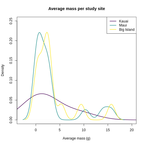
It looks like Kauai insects have a smoother distribution of body masses, while Maui and Big Island show more clumped distributions, possibly due to higher immigration on those islands.
Hill numbers
Hill numbers are a useful and informative summary of trait diversity,
in addition to other biodiversity variables (Gaggiotti
et al. 2018). They contain signatures of the processes underlying
community assembly. To calculate Hill numbers for traits, you’re going
to use the hill_func() function from the hillR
package. It requires two inputs- the site by species abundance dataframe
and a traits dataframe that has species as rows and traits as
columns.
R
abundances_wide <- pivot_wider(
    abundances,
    id_cols = site,
    names_from = final_name,
    values_from = abundance,
    values_fill = 0
)

# tibbles don't like row names
abundances_wide <- as.data.frame(abundances_wide)

row.names(abundances_wide) <- abundances_wide$site

# remove the site column
abundances_wide <- abundances_wide[,-1]
Now, to create the traits dataframe for Hill number calculations purposed, we just need the taxonomic names and trait mean.
R
traits_simple <- traits_sumstats[, c("final_name", "mean_mass_g")]

head(traits_simple)
OUTPUT
            final_name mean_mass_g
1         Cis signatus  2.75162128
2 Acanthia procellaris  1.09171586
3     Spolas solitaria  3.01819088
4        Laupala pruna  0.05259815
5  Toxeuma hawaiiensis  2.16818518
6  Chrysotus parthenus  1.76717404
Next, you need to filter for unique species in the dataframe.
R
traits_simple <- unique(traits_simple)

head(traits_simple)
OUTPUT
            final_name mean_mass_g
1         Cis signatus  2.75162128
2 Acanthia procellaris  1.09171586
3     Spolas solitaria  3.01819088
4        Laupala pruna  0.05259815
5  Toxeuma hawaiiensis  2.16818518
6  Chrysotus parthenus  1.76717404
Finally, you need to set the species names to be row names and remove
the final_name column. Note, you have to use the
drop = FALSE argument because R has the funny behavior that
it likes to convert single-column dataframes into a vector.
R
row.names(traits_simple) <- traits_simple$final_name

traits_simple <- traits_simple[, -1, drop = FALSE]

head(traits_simple)
OUTPUT
                     mean_mass_g
Cis signatus          2.75162128
Acanthia procellaris  1.09171586
Spolas solitaria      3.01819088
Laupala pruna         0.05259815
Toxeuma hawaiiensis   2.16818518
Chrysotus parthenus   1.76717404
Next, you’ll use the hill_func() function from the
hillR package to calculate Hill numbers 0-2 of body size
across sites.
R
traits_hill_0 <- hill_func(comm = abundances_wide, traits = traits_simple, q = 0)

traits_hill_1 <- hill_func(comm = abundances_wide, traits = traits_simple, q = 1)

traits_hill_2 <- hill_func(comm = abundances_wide, traits = traits_simple, q = 2)
The output of hill_func() returns quite a few Hill
number options, which are defined in Chao
et al. 2014. For simplicity’s sake, we will look at
D_q, which from the documentation is the:
> functional Hill number, the effective number of equally abundant and functionally equally distinct species
R
traits_hill_1
OUTPUT
          BI_01      MA_01      KA_01
Q     0.7949925   5.049335   14.11121
FDis  0.5983183   4.283883   10.90624
D_q   7.7865058  13.561339   10.07768
MD_q  6.1902140  68.475746  142.20828
FD_q 48.2001378 928.622813 1433.12950
To gain an intuition for what this means, let’s plot our data. First, you will wrangle the output into a single dataframe to work with. Since Hill q = 0 is species richness, let’s focus on Hill q = 1 and Hill q = 2.
R
traits_hill <- data.frame(hill_trait_0 = traits_hill_0[3, ],
                          hill_trait_1 = traits_hill_1[3, ],
                          hill_trait_2 = traits_hill_2[3, ])

# I don't like rownames for plotting, so making the rownames a column
traits_hill <- cbind(site = rownames(traits_hill), traits_hill)

rownames(traits_hill) <- NULL

traits_hill
OUTPUT
   site hill_trait_0 hill_trait_1 hill_trait_2
1 BI_01     29.03417     7.786506     4.722840
2 MA_01     15.78844    13.561339    12.185382
3 KA_01     20.04110    10.077680     7.094183
Let’s look at how Hill q = 1 compare across sites.
R
plot(factor(traits_hill$site, levels = c("KA_01", "MA_01", "BI_01")),
     traits_hill$hill_trait_1, ylab = "Hill q = 1")
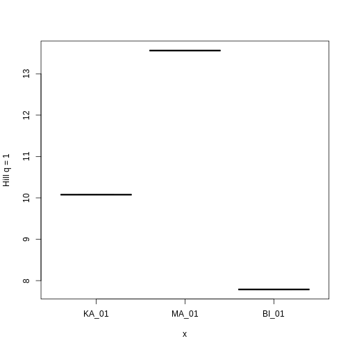
Hill q = 1 is smallest on the Big Island, largest on Maui, and in the middle on Kauai. But what does this mean? To gain an intuition for what a higher or lower trait Hill number means, you will make rank plots of the trait data, to make a plot analogous to the species abundance distribution.
R
# figure out max number of species at a site for axis limit setting below
max_sp <- sapply(traits_sumstats_split, nrow)
max_sp <- max(max_sp)


plot(
    sort(traits_sumstats_split$KA_01$mean_mass_g, decreasing = TRUE),
    main = "Average mass per study site",
    xlab = "Rank",
    ylab = "Average mass (mg)",
    pch = 19,
    col = "#440154FF",
    xlim = c(1, max_sp),
    ylim = c(0, max(traits_simple$mean_mass_g))
)

points(
    sort(traits_sumstats_split$MA_01$mean_mass_g, decreasing = TRUE),
    pch = 19,
    col = "#21908CFF"
)

points(
    sort(traits_sumstats_split$BI_01$mean_mass_g, decreasing = TRUE),
    pch = 19,
    col = "#FDE725FF"
)

legend(
    "topright",
    legend = c("Kauai", "Maui", "Big Island"),
    pch = 19,
    col = c("#440154FF", "#21908CFF", "#FDE725FF")
)
You can see clearly that the trait distributions differ across islands, where Maui has more species than the other islands and a seemingly more even distribution than Kauai. Kauai seems to have a greater spread of trait values, however, species abundance strongly influences the calculation of a Hill number. To visualize the role of abundance, we can replicate each species mean by the abundance of that species
R
# replicate abundances
biIndividualsTrt <- rep(traits_sumstats_split$BI_01$mean_mass_g,
                        traits_sumstats_split$BI_01$abundance)
maIndividualsTrt <- rep(traits_sumstats_split$MA_01$mean_mass_g,
                        traits_sumstats_split$MA_01$abundance)
kaIndividualsTrt <- rep(traits_sumstats_split$KA_01$mean_mass_g,
                        traits_sumstats_split$KA_01$abundance)


plot(
    sort(kaIndividualsTrt, decreasing = TRUE),
    main = "Average mass across individuals",
    xlab = "Rank",
    ylab = "Average mass (mg)",
    pch = 19,
    col = "#440154FF",
    ylim = c(0, max(traits_simple$mean_mass_g))
)

points(
    sort(maIndividualsTrt, decreasing = TRUE),
    pch = 19,
    col = "#21908CFF"
)

points(
    sort(biIndividualsTrt, decreasing = TRUE),
    pch = 19,
    col = "#FDE725FF"
)

legend(
    "topright",
    legend = c("Kauai", "Maui", "Big Island"),
    pch = 19,
    col = c("#440154FF", "#21908CFF", "#FDE725FF")
)
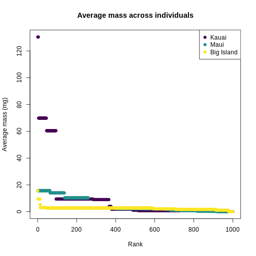
What we can see from the individuals-level plot is that much of the range of trait values on Kauai are brought by very rare species, these rare species do not contribute substantially to the diversity as expressed by Hill numbers.
Content from Summarizing phylogenetic data
Last updated on 2023-07-11 | Edit this page
Overview
Questions
- What biological information is stored in phylogenetic Hill numbers?
- How do you import and manipulate phylogeny data in R?
- What are the common phylogeny data formats?
- How do you visualize phylogenies in R?
- How do you calculate Hill numbers with phylogenetic data?
Objectives
After following this episode, participants will be able to:
- Identify key features of the Newick format
- Import and manipulate phylogenetic data in the R environment
- Visualize phylogenies
- Calculate and interpret phylogenetic Hill numbers
Introduction to phylogenetic data
In this episode, we will explore how to extract information from phylogenetic trees in order to complement our hypotheses and inferences about processes shaping biodiversity patterns. Phylogenetic trees have information about how the species in a taxonomic group are related to each other and how much relative evolutionary change has accumulated among them. Since local communities differ in their phylogenetic composition, this information can give insights on why communities are how they are.
The relative phylogenetic distance among species in a community as well as the distribution of the amount of evolutionary history (represented by the length of the branches in a phylogeny) are a result of different factors such as the age since the initial formation of the community and the rate of macroevolutionary processes such as speciation and extinction. For instance, young communities that are dominated by closely related species and show very short branch lengths may suggest a short history with few colonization events and high rates of local speciation; alternatively, if the same young communities harbor distantly related species with longer branch lengths, it may suggest that most of the local diversity was generated by speciation elsewhere followed by colonization events involving distantly related species. Coupled with information on ecological traits and rates of macroevolutionary processes, these patterns also allow to test for hypotheses regarding, for instance, ecological filtering or niche conservatism.
Summarizing this phylogenetic information (i.e., phylogenetic distance and distribution of branch lengths) is therefore important for inference. As we have seen in previous episodes, the use of Hill numbers is an informative approach to summarize biodiversity. In this episode, we will see how phylogenetic Hill numbers in different orders are able to capture information about 1) the total amount of evolutionary history in different communities; 2) how this history is relatively distributed across the community.
Working with phylogenetic data in R
Importing phylogenetic data
Several file formats exist to store phylogenetic information. The
most common formats are the Newick and Nexus
formats. Both these formats are plain text files storing different
levels of information about the taxa relationship and evolutionary
history. Newick files are the standard for representing
trees in a computer-readable form, as they can be extremely simple and
therefore do not take up much memory. Nexus file, on the
other hand, are composed by different blocks regarding different types
of information and can be used to store DNA alignments, phylogenetic
trees, pre-defined groupings of taxa, or everything at once. Since they
are a step ahead in complexity, we will stick with Newick
files for now.
Newick files store the information about the clades in a
tree by representing each clade within a set of parentheses. Sister
clades are separated by ,. The notation also requires us to
add the symbol ; to represent the end of the information
for that phylogenetic tree.
The basic structure of a tree in a Newick format is
therefore as follows:
((A,B),C);
The notation above indicates that: 1. we have three taxa in our tree,
named A, B and C; 2.
A and B form one clade (A,B); 3. the (A,B)
clade is sister to the C clade (we represent that by adding
another set of parentheses and a , separating (A,B) from
C).
In addition, Newick files can also store information on
the branch leading to it tip and node. We do that by adding
: after each tip/node.
((A:0.5,B:0.5):0.5,C:1);
The notation above indicates that: 1. the branches containing A and B have each a length = 0.5; 2. the branch that leads to the node connecting A and B also has length = 0.5; 3. the branch leading to C has length = 1.
The notation above is what we import into R to start working with and manipulating our phylogenetic tree. For that goal, we will use the ape package. Below, we are also loading a few other packages we’ll be using later on.
R
library(ape)
library(tidyr)
library(hillR)
To import our tree, we will be using the function
read.tree() from the ape package. In the case
of simple trees as the one above, we could directly create them within R
by giving that notation as a character value to this
function, using the text argument, as shown below:
R
example_tree <- read.tree(text = '((A:0.5,B:0.5):0.5,C:1);')
Now, we can visually inspect our tree using the plot()
function:
R
plot(example_tree)
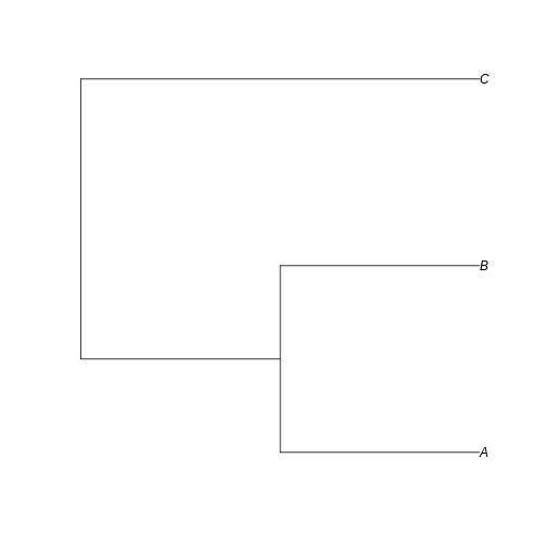
Can you visualize the text notation in that image? We can see the same information: A is closer related to B than C, and the branches leading to A and B have half the length of the branch leading to C.
The read.tree() function creates an object of class
phylo. We can further investigate this object by calling it
in our console:
R
example_tree
OUTPUT
Phylogenetic tree with 3 tips and 2 internal nodes.

Tip labels:
  A, B, C

Rooted; includes branch lengths.
The printed information shows us that we have a phylogenetic tree with 3 tips and 2 internal nodes, where the tip labels are “A, B, C”. We also are informed that this tree is rooted and has branch lengths.
One way to access the components of this object and better explore it
is to use $ after the object name. Here, it will be
important for us to know a little bit more about where the information
about tip labels and branch lengths are stored in that
phylo object. Easy enough, we can access that by calling
tip.labels and edge.length after
$.
R
example_tree$tip.label
OUTPUT
[1] "A" "B" "C"R
example_tree$edge.length
OUTPUT
[1] 0.5 0.5 0.5 1.0Cleaning and filtering phylogenetic data
Now that we learned how to import and visualize trees in R, let’s bring the phylogeny for the communities we are working with in this workshop. Our data so far consists of abundances and traits of several taxa of arthropods collected across three islands in the Hawaiian archipelago. Let’s work though importing phylogenetic information for these species.
Two common approaches to retrieving a phylogeny for a focal group are
1) relying on a published phylogeny for the group, or 2) surveying
public phylogenetic databases based on your taxa list. A common option
for the latter is the Open
Tree of Life Taxonomy, a public database that synthesizes taxonomic
information from different sources. You can even interact with this
database using the R package rotl. A few tutorials to do so
exist online, like this one.
Using a public database is a good approach when working with taxonomic
groups that are not heavily investigated regarding their phylogenetic
relationships (the well-known Darwinian
shortfall). In such cases, databases like OTL will give you a
summary phylogeny already filtered for the taxa you have in hand and
cross-checked for synonyms and misspellings.
For this workshop, since we are using simulated data, we will work
with the first option: a “published” arthropod phylogeny. Let’s load
this phylogeny into R using the function read.tree we
learned earlier.
R
arthro_tree <- read.tree('https://raw.githubusercontent.com/role-model/multidim-biodiv-data/main/episodes/data/phylo_raw.nwk')

class(arthro_tree)
OUTPUT
[1] "phylo"This new phylo object is way larger than the previous
one, being a “real” phylogeny and all. You can inspect it again by
directly calling the object arthro_tree. To plot it, we
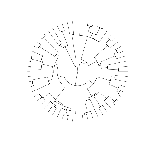
will use the type argument to modify how our tree will be
displayed. Here, we used the option 'fan', to display a
circular phylogeny (slightly better to show such a large phylogeny in
the screen). We also set the show.tip.label argument to
False.
R
plot(arthro_tree, type = 'fan', show.tip.label = F)
How do we combine all this information with the community datasets we have so far for our three islands? First, we will have to perform some name checking and filtering.
Cleaning and checking phylogeny taxa
The first thing we want to do is to check the tip labels in our tree. Since this is a “published” arthropod phylogeny, we will likely not have any misspelling in the tip names of the object. However, it is always good practice to check contents to see if anything weird stands out.
R
arthro_tree$tip.label
OUTPUT
 [1] "Leptogryllus_fusconotatus"   "Hylaeus_facilis"
 [3] "Laupala_pruna"               "Eurynogaster_vittata"
 [5] "Cydia_gypsograpta"           "Toxeuma_hawaiiensis"
 [7] "Proterhinus_punctipennis"    "Drosophila_quinqueramosa"
 [9] "Ectemnius_mandibularis"      "Nesodynerus_mimus"
[11] "Proterhinus_xanthoxyli"      "Nesiomiris_lineatus"
[13] "Aeletes_nepos"               "Scaptomyza_vagabunda"
[15] "Agrotis_chersotoides"        "Kauaiina_alakaii"
[17] "Atelothrus_depressus"        "Metrothorax_deverilli"
[19] "Scaptomyza_villosa"          "Hylaeus_sphecodoides"
[21] "Lucilia_graphita"            "Xyletobius_collingei"
[23] "Hyposmocoma_sagittata"       "Cis_signatus"
[25] "Hyposmocoma_scolopax"        "Dryophthorus_insignoides"
[27] "Eudonia_lycopodiae"          "Chrysotus_parthenus"
[29] "Limonia_sabroskyana"         "Hyposmocoma_marginenotata"
[31] "Mecyclothorax_longulus"      "Deinomimesa_haleakalae"
[33] "Trigonidium_paranoe"         "Eudonia_geraea"
[35] "Drosophila_furva"            "Hyposmocoma_geminella"
[37] "Drosophila_obscuricornis"    "Campsicnemus_nigricollis"
[39] "Odynerus_erythrostactes"     "Phaenopria_soror"
[41] "Gonioryctus_suavis"          "Laupala_vespertina"
[43] "Acanthia_procellaris"        "Odynerus_caenosus"
[45] "Elmoia_lanceolata"           "Nesodynerus_molokaiensis"
[47] "Sierola_celeris"             "Nysius_lichenicola"
[49] "Parandrita_molokaiae"        "Agonismus_argentiferus"
[51] "Cephalops_proditus"          "Nesomicromus_haleakalae"
[53] "Lispocephala_dentata"        "Agrion_nigrohamatum"
[55] "Plagithmysus_ilicis_ekeanus" "Scatella_clavipes"
[57] "Hedylepta_accepta"           "Cis_bimaculatus"
[59] "Hydriomena_roseata"          "Spolas_solitaria"
And indeed we find something: even though there are probably no
misspellings, the genus and species name in this tree are separated by
an underscore symbol _. Since the names in our
site-by-species matrix do not have that underscore, we will get an error
when matching the data if we don’t fix this spelling.
One useful function to do this fixing is the function
gsub(). This function allows you to look for a specific
character pattern inside character objects, and replace them by any
other pattern you may want. In our case, we have a vector of 60
character values containing the names of our tips. We want to find the
_ character inside each character value and replace it by
an empty space, so it becomes equal to what we have in our
site-by-species matrix. We do so by providing to the gsub()
function: 1) the pattern we want to replace; 2) the new pattern we want
to replace it with; 2) the character object or vector containing the
values to be searched. Finally, we assign the output of that function
back to the tip.label slot in the arthro_tree
object.
R
arthro_tree$tip.label <- gsub('_',' ',arthro_tree$tip.label)

# A quick check to see if worked
arthro_tree$tip.label
OUTPUT
 [1] "Leptogryllus fusconotatus"   "Hylaeus facilis"
 [3] "Laupala pruna"               "Eurynogaster vittata"
 [5] "Cydia gypsograpta"           "Toxeuma hawaiiensis"
 [7] "Proterhinus punctipennis"    "Drosophila quinqueramosa"
 [9] "Ectemnius mandibularis"      "Nesodynerus mimus"
[11] "Proterhinus xanthoxyli"      "Nesiomiris lineatus"
[13] "Aeletes nepos"               "Scaptomyza vagabunda"
[15] "Agrotis chersotoides"        "Kauaiina alakaii"
[17] "Atelothrus depressus"        "Metrothorax deverilli"
[19] "Scaptomyza villosa"          "Hylaeus sphecodoides"
[21] "Lucilia graphita"            "Xyletobius collingei"
[23] "Hyposmocoma sagittata"       "Cis signatus"
[25] "Hyposmocoma scolopax"        "Dryophthorus insignoides"
[27] "Eudonia lycopodiae"          "Chrysotus parthenus"
[29] "Limonia sabroskyana"         "Hyposmocoma marginenotata"
[31] "Mecyclothorax longulus"      "Deinomimesa haleakalae"
[33] "Trigonidium paranoe"         "Eudonia geraea"
[35] "Drosophila furva"            "Hyposmocoma geminella"
[37] "Drosophila obscuricornis"    "Campsicnemus nigricollis"
[39] "Odynerus erythrostactes"     "Phaenopria soror"
[41] "Gonioryctus suavis"          "Laupala vespertina"
[43] "Acanthia procellaris"        "Odynerus caenosus"
[45] "Elmoia lanceolata"           "Nesodynerus molokaiensis"
[47] "Sierola celeris"             "Nysius lichenicola"
[49] "Parandrita molokaiae"        "Agonismus argentiferus"
[51] "Cephalops proditus"          "Nesomicromus haleakalae"
[53] "Lispocephala dentata"        "Agrion nigrohamatum"
[55] "Plagithmysus ilicis ekeanus" "Scatella clavipes"
[57] "Hedylepta accepta"           "Cis bimaculatus"
[59] "Hydriomena roseata"          "Spolas solitaria"
Now that we fixed this first obvious issue, we can start looking for others. Since we want to calculate phylogenetic diversity for each of our communities, our main concern here is to make sure that all taxa present in our communities can be found in this phylogeny. One important issue that may arise is the use of different names for the same taxa across the two datasets (i.e., synonyms). This is especially important since we previouslu performed a synonym check and cleaning in our abundance dataset; we need to make sure the names in our tree will follow the same nomenclature decisions.
To see if there are any mismatches, let’s first retrieve a list of
the names in our abundances dataset. Since this dataset has repeated
instances of the same species when it shows up in different islands, we
wrap the vector of taxa names in the function unique() to
return each species name only once.
R
all_names <- unique(abundances$final_name)
To cross-check this list against the list of names in our phylogeny,
we can use the Boolean operator %in% coupled with
!. This will allow us to check for names present in
all_names that are not included in the
arthro_tree$tip.label. In summary, the expression
A %in% B would return whether each element of vector A is
present in vector B. This is returned as a Boolean vector: if
TRUE, the element of that position in A exists in B; if
FALSE, it does not. We add the ! (NOT)
operator to return the opposite of that expression, in a way that
!(A %in% B) will return whether each element of vector A is
NOT present in vector B. In this case, every time we see
TRUE, it means the element in that position is NOT
in vector B.
R
not_found <- !(all_names %in% (arthro_tree$tip.label))
not_found
OUTPUT
 [1] FALSE FALSE FALSE FALSE FALSE FALSE FALSE FALSE FALSE FALSE FALSE  TRUE
[13] FALSE FALSE FALSE FALSE FALSE FALSE FALSE FALSE FALSE FALSE FALSE FALSE
[25] FALSE FALSE FALSE FALSE FALSE FALSE FALSE
Checking the vector not_found, we can see it is a
collection of TRUEs and FALSEs. We can use that vector to perform
bracket subsetting in the vector all_names. Doing so, we
are retrieving from all_names only the elements in the
position where not_found is TRUE.
R
all_names[not_found]
OUTPUT
[1] "Peridroma chersotoides"The expression above give us the one element of
all_names that is not present in
arthro_tree$tip.label. As we expected, it is a synonym that
we corrected in our abundances
episode. Our tree still has the old name Agrotis chersotoides
whereas our site-by-species matrix has the updated name Peridroma
chersotoides. To correct that, we need to modify the tip label in
our tree to match the new name. How can we do that?
Challenge
Modify the old name Agrotis chersotoides in our phylogenetic tree, replacing it by Peridroma chersotoides. To do so, you will need to 1) find the position of the old name in labels in our tree; 2) assign the new name in the right position where the old name is.
Hint: a similar task was performed before in the abundances.
We need to perform an assignment operation in the position where the
old name is located inside arthro_tree$tip.label. To find
that position, we can use Boolean matching to ask which element of
arthro_tree$tip.label equals the old name.
R
arthro_tree$tip.label[arthro_tree$tip.label == 'Agrotis chersotoides'] <- "Peridroma chersotoides"
A good practice after correcting the name is to re-check if all names
in our abundance dataset match the names in the phylogeny. This time, we
expect all elements in the vector not_found to be
FALSE. We can use the function which() to ask
“which elements in not_found are TRUE We
expect the answer to be an empty vector, indicating”no elements in
not_found are TRUE“.
R
not_found <- !(all_names %in% (arthro_tree$tip.label))
which(not_found)
OUTPUT
integer(0)Pruning our phylogeny
Now that we have a modified tree where all taxa names are present in our abundances dataset, we can work on pruning our phylogeny to the taxa present in our communities. This is especially important when working with published phylogenies as these are usually large files containing several taxa that may not exist in the local community.
We can prune our phylogeny using the function keep.tip()
from the ape package. For this function, we provide the
entire phylogeny plus the names of the tips we want to keep. Here, we
will retrieve those names from the abundances dataset.
R
arthro_tree_pruned <- keep.tip(arthro_tree,abundances$final_name)
With a pruned phylogeny and a site-by-species matrix, we have the two bits of information we need to summarize phylogenetic diversity per community. As we saw in previous episodes, we can use such abundance matrix to calculate Hill numbers and help us compare patterns across the different communities. In the traits episode, we saw how we can combine abundance and trait data to extract Hill numbers as values that summarize the distribution of trait variation across communities. Here we will be following the same approach to summarize the amount and the distribution of evolutionary history across the species in our community.
Summarizing with hill numbers
In this section, we will extract some summary statistics about the pattern of phylogenetic diversity (PD) in our communities. As we discussed in the intro of this episode, the relative phylogenetic distance among species and the distribution of this distance can give insights into processes of community assembly. Here, we will make use of Hill numbers to extract summaries of phylogenetic distances, i.e. the length of the branches in the phylogenetic tree leading to the taxa present in each community. Phylogenetic hill numbers incorporate information on both the phylogenetic structure of a system and the abundances of different species. In order to get an intuition for how these different components influence phylogenetic hill numbers, we’ll set our Hawaiian data aside for a moment and first explore the behavior of this summary statistic using a few simplified example datasets.
Example 1. Trees with different branch lenghts
For our examples, we’ll assume we have one single community with
eight taxa: A through H. Let’s create two site-by-species matrix for
this community: one denoting even abundance across species, and another
one with uneven abundance. For the even communitu, we create a vector of
the value 1 repeated 8 times; for the uneven community,
we’ll create a vector where abundance goes up from species A to species
H (for simplicity, we’ll just use values from 1 to 8). We then transform
them to dataframe, and name the columns with the names of the
species.
R
even_comm <- data.frame(rbind(rep(1,8))) # Abundance = 1 for all species
uneven_comm <- data.frame(rbind(seq(1,8))) # Abundance equal 1 for species A and goes up to 8 towards species H.

# We name the columns with the species names
colnames(even_comm) <- colnames(uneven_comm) <- c('A','B','C','D','E','F','G','H')
Now let’s create two different possible trees for these communities: one with short branch lengths and another with longer branch lengths. Remember: branch length = amount of evolutionary change
R
short_tree <- read.tree(text='(((A:3,B:3):1,(C:3,D:3):1):1,((E:3,F:3):1,(G:3,H:3):1):1);')
long_tree <- read.tree(text='(((A:6,B:6):1,(C:6,D:6):1):1,((E:6,F:6):1,(G:6,H:6):1):1);')
If we plot both trees…
R
plot(short_tree)
R
plot(long_tree)
…we can see that the branches leading to extant taxa are longer for
long_tree, as we intended. This suggests that a greater
amount of evolutionary change is happening in these recent branches of
the longer tree when compared to the shorter tree.
Now, we will calculate phylogenetic hill numbers for both trees using
both even and uneven communities. To store the calculated values, we’ll
create a data.frame called even_comm_short_tree. The first
column will be our Hill numbers to be calculated; the second column will
be the Hill number order from 0 to 3, to see how the order affects the
values; the third and fourth column will be the description of our
components
R
even_comm_short_tree <- data.frame(
    hill_nb = NA,
    q = 0:3,
    comm = "even",
    tree = "short"
)
Now we will use a for loop to calculate phylogenetic
Hill numbers using the hill_phylo function from the
hillR package. This function takes in a a site-by-species
matrix and phylogeny, and returns phylogenetic Hill numbers for each
site based on which species are present there. We provide to the
function the site-by-species matrix, the phylogenetic tree and the
order.
R
for(i in 1:nrow(even_comm_short_tree)) {
    even_comm_short_tree$hill_nb[i] <- hill_phylo(even_comm, short_tree, q = even_comm_short_tree$q[i])
}
Let’s repeat this process for the longer tree:
R
even_comm_long_tree <- data.frame(
    hill_nb = NA,
    q = 0:3,
    comm = "even",
    tree = "long"
)

for(i in 1:nrow(even_comm_long_tree)) {
    even_comm_long_tree$hill_nb[i] <- hill_phylo(even_comm, long_tree, q = even_comm_long_tree$q[i])
}
We can combine both dataframes and plot the values for comparison:
R
even_comm_nb <- data.frame(rbind(even_comm_short_tree,even_comm_long_tree))

plot(even_comm_nb$q[even_comm_nb$tree=='short'],
     even_comm_nb$hill_nb[even_comm_nb$tree=='short'],
     type='b',col='red',
     xlab = 'Order',ylab='Hill values',
     xlim = range(even_comm_nb$q),
     ylim = range(even_comm_nb$hill_nb))

lines(even_comm_nb$q[even_comm_nb$tree=='long'],
     even_comm_nb$hill_nb[even_comm_nb$tree=='long'],
     type='b',col='darkred')
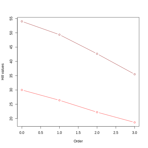
This figure clearly shows that the tree with longer branches (dark red line) harbors higher evolutionary history, and therefore higher PD, as calculated by Hill numbers. It also shows that the Hill number value decreases as the order goes up, since higher orders focus on branch lengths that are more common.
What would happen if the abundance of species in our community was uneven (a more realistic scenario)? In this case, both branch lengths and how abundant each branch is will have an effect on the calculated value. To visualize, let’s repeat the calculations above for the uneven community.
R
# Uneven comm with short tree
uneven_comm_short_tree <- data.frame(
    hill_nb = NA,
    q = 0:3,
    comm = "uneven",
    tree = "short"
)

for(i in 1:nrow(uneven_comm_short_tree)) {
    uneven_comm_short_tree$hill_nb[i] <- hill_phylo(uneven_comm, short_tree, q = uneven_comm_short_tree$q[i])
}

# Uneven comm with long tree
uneven_comm_long_tree <- data.frame(
    hill_nb = NA,
    q = 0:3,
    comm = "uneven",
    tree = "long"
)

for(i in 1:nrow(uneven_comm_long_tree)) {
    uneven_comm_long_tree$hill_nb[i] <- hill_phylo(uneven_comm, long_tree, q = uneven_comm_long_tree$q[i])
}

# Combining results
uneven_comm_nb <- data.frame(rbind(uneven_comm_short_tree,uneven_comm_long_tree))
Let’s plot all results together, using red colors for even communities and blue colors for uneven community. Ligher colors will represent short trees whereas darker colors will represent long trees.
R
plot(even_comm_nb$q[even_comm_nb$tree=='short'],
     even_comm_nb$hill_nb[even_comm_nb$tree=='short'],
     type='b',col='red',
     xlab = 'Order',ylab='Hill values',
     xlim = range(even_comm_nb$q),
     ylim = range(min(uneven_comm_nb$hill_nb),max(even_comm_nb$hill_nb)))

lines(even_comm_nb$q[even_comm_nb$tree=='long'],
     even_comm_nb$hill_nb[even_comm_nb$tree=='long'],
     type='b',col='darkred')

lines(uneven_comm_nb$q[uneven_comm_nb$tree=='short'],
     uneven_comm_nb$hill_nb[uneven_comm_nb$tree=='short'],
     type='b',col='lightblue')

lines(uneven_comm_nb$q[uneven_comm_nb$tree=='long'],
     uneven_comm_nb$hill_nb[uneven_comm_nb$tree=='long'],
     type='b',col='darkblue')
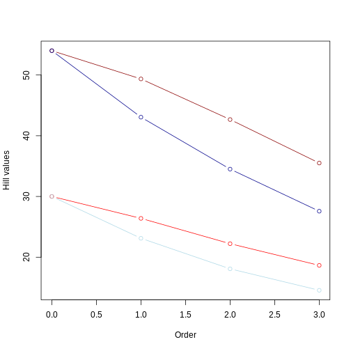
From this picture, we can take a few insights:
Longer branches still yield higher Hill numbers, regardless of the evenness in the community abundance;
The Hill number for q = 0 remains the same, regardless of the evenness.
As already observed, the value of the hill numbers drop as the order goes up. In the even community, since species have the same abundance, this decrease reflects higher orders focusing on more common values of branch lengths. In the uneven community, where species have different abundances, this decrease reflects higher orders focusing less and less on branches leading to rare taxa.
For q = 1 to 3, Hill numbers are always lower for uneven communities. This suggests that although branch lengths are the same (e.g., both dark red and dark blue lines represent the long tree), these branches are unevenly represented in the community due to uneven abundance of species. This unevenness is represented by the lower values of Hill number on higher orders. In other words, some branches in the tree “dominate” the community more than others. We can summarize this by saying that the higher the unevenness the lower the value of the Hill number will be.
Keypoints
-
hillRcalculates phylogenetic hill numbers given a phylogeny and a site by species matrix. - In trees with a similar topology, phylogenetic Hill number of order 0 reflect the sum of branch lengths. Orders of 1 and higher reflect the sum of branch lengths weighted by the relative abundance of different species.
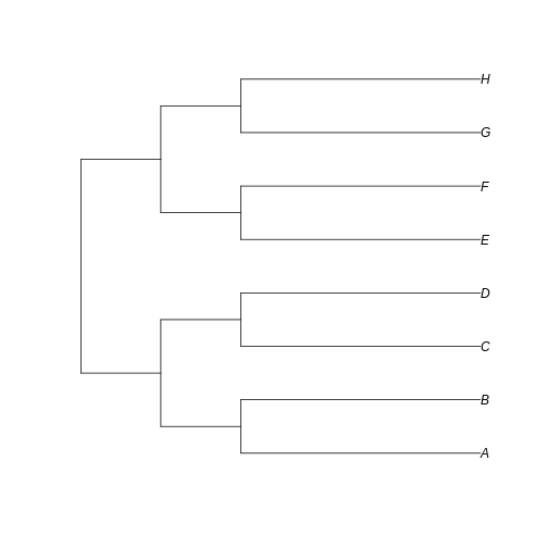
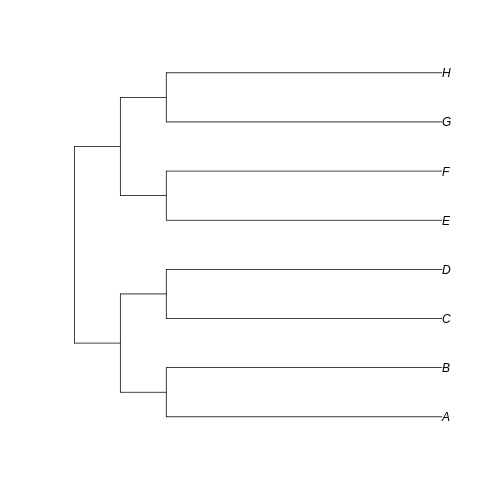
Example 2. Balanced vs unbalanced trees
So far, we have learned that Hill numbers are affected by both the sum of branch lengths and the relative representation of each branch (in terms of species abundance) in the community. For example 1, we have used a perfectly balanced tree, i.e., all extant taxa have equal branch length. In example 2, we will explore the effects of the uneven distribution of cladogenesis event along the tree, leading to different phylogeny structures.
Let’s create a totally balanced tree…
R
balanced_tree <- read.tree(text='(((A:1,B:1):1,(C:1,D:1):1):1,((E:1,F:1):1,(G:1,H:1):1):1);')
… and a totally unbalanced tree.
R
unbalanced_tree <- read.tree(text='(A:7,(B:6,(C:5,(D:4,(E:3,(F:2,(G:1,H:1):1):1):1):1):1):1);')
Let’s plot both trees for comparison:
R
plot(balanced_tree)
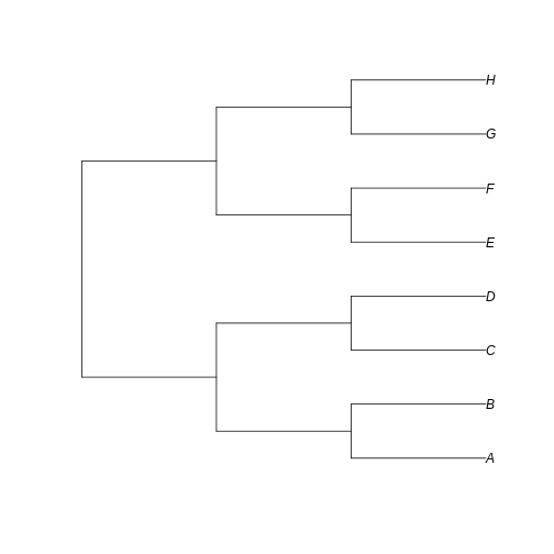
R
plot(unbalanced_tree)
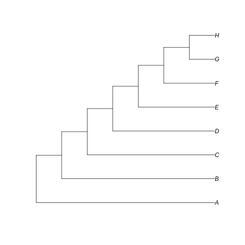
Notice that here the difference between the trees resides in the fate of each new lineage at a node. In the unbalanced uneven tree, at each diversification event one of the lineages always persists till the present with no change while the other undergoes another round of diversification. In the even tree, both lineages from each node undergo a new split. The consequence is that in the even tree, all extant species result from recent diversification (i.e., they have a short evolutionary history before coalescing into their ancestor), whereas in the unbalanced tree we have a mix of old and recent lineages. This means that the phylogenetic history itself is creating an uneven representation of branch lengths across the community (even before we account for species abundance)
To see how such phylogenetic structure influences hill numbers, let’s repeat the calculations from example 1 with these new trees. First, let’s focus on the even community (i.e., not introducing the relative species abundance factor yet):
R
even_comm_balanced_tree <- data.frame(
    hill_nb = NA,
    q = 0:3,
    comm = "even",
    tree = "balanced"
)

for(i in 1:nrow(even_comm_balanced_tree)) {
    even_comm_balanced_tree$hill_nb[i] <- hill_phylo(even_comm, balanced_tree, q = even_comm_balanced_tree$q[i])
}

even_comm_unbalanced_tree <- data.frame(
    hill_nb = NA,
    q = 0:3,
    comm = "even",
    tree = "unbalanced"
)

for(i in 1:nrow(even_comm_unbalanced_tree)) {
    even_comm_unbalanced_tree$hill_nb[i] <- hill_phylo(even_comm, unbalanced_tree, q = even_comm_unbalanced_tree$q[i])
}

even_comm_nb <- data.frame(rbind(even_comm_balanced_tree,even_comm_unbalanced_tree))

plot(even_comm_nb$q[even_comm_nb$tree=='balanced'],
     even_comm_nb$hill_nb[even_comm_nb$tree=='balanced'],
     type='b',col='red',
     xlab = 'Order',ylab='Hill values',
     xlim = range(even_comm_nb$q),
     ylim = range(even_comm_nb$hill_nb))

lines(even_comm_nb$q[even_comm_nb$tree=='unbalanced'],
     even_comm_nb$hill_nb[even_comm_nb$tree=='unbalanced'],
     type='b',col='darkred')
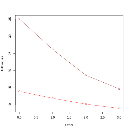
This plot is similar to example 1 in two ways: 1) one of the trees has higher hill number values, in this case the unbalanced tree. This suggests that the unbalanced structure of the tree accounts for a deeper evolutionary history (i.e., lineages have overall longer branches); 2) the value of the hill numbers drop as the order goes up. This happens because higher orders are weighting less and less those branch lengths that are not so common (like, for instance, the short branch lengths in the unbalanced tree).
Something new that we observe here is a more evident difference between trees in the rate of change of the Hill number value as we increase the order. The unbalanced tree (darker red) shows a steeper drop than the balanced tree (lighter red). This is similar to what we observed in the abundances episode: uneven communities show a steeper drop in Hill numbers as order increases. In this example, instead of species abundance, the unevenness of the community is represented by the structure of the phylogeny: a completely unbalanced tree combining long and short branches generates an unevenness in the distribution of branch lengths. Notice that this difference in rate of change barely observed in example 1: when plotting two trees with the same structure (short vs long trees, but both fully balanced), the lines are very similar In example 1, the difference in the rate of change only becomes evident when we incorporate unevenness from the species abundance, but here in example 2 we see this difference deriving already from the different structures of the trees.
If the tree structure is already introducing some unevenness in our community, how would the pattern differ when species relative abundance is included?
In this case, both the structure of the tree and the species abundance interact to generate a pattern of unevenness. Specifically, the overall value of PD will be the sum of branch lengths weighted by their abundance in the community as informed by the species abundance distribution (instead of by the frequency of the branch length in the tree). This added information brings new insights. It may be the case, for instance, that in the unbalanced tree, even though long branches are over represented, maybe the species with long branches are actually super rare in our community, and the short-branch species are actually super abundant. As you can probably infer, this difference suggests something about the evolutionary history of our community, in this case that the most abundant species have a very recent evolutionary history. Similarly, even though branch lengths are the same in the balanced tree, if some of the species is more abundant than others, it suggests that the evolutionary history of the tree is unevenly represented in our community.
To visualize these interaction between tree structure and species relative abundance, let’s redo the calculation for Hill numbers with balanced and unbalanced trees, this time using the uneven community. We’ll plot all final values together for comparison.
R
uneven_comm_balanced_tree <- data.frame(
    hill_nb = NA,
    q = 0:3,
    comm = "uneven",
    tree = "balanced"
)

for(i in 1:nrow(uneven_comm_balanced_tree)) {
    uneven_comm_balanced_tree$hill_nb[i] <- hill_phylo(uneven_comm, balanced_tree, q = uneven_comm_balanced_tree$q[i])
}

uneven_comm_unbalanced_tree <- data.frame(
    hill_nb = NA,
    q = 0:3,
    comm = "uneven",
    tree = "unbalanced"
)

for(i in 1:nrow(uneven_comm_unbalanced_tree)) {
    uneven_comm_unbalanced_tree$hill_nb[i] <- hill_phylo(uneven_comm, unbalanced_tree, q = uneven_comm_unbalanced_tree$q[i])
}

uneven_comm_nb <- data.frame(rbind(uneven_comm_balanced_tree,uneven_comm_unbalanced_tree))

plot(even_comm_nb$q[even_comm_nb$tree=='balanced'],
     even_comm_nb$hill_nb[even_comm_nb$tree=='balanced'],
     type='b',col='red',
     xlab = 'Order',ylab='Hill values',
     xlim = range(even_comm_nb$q),
     ylim = range(min(uneven_comm_nb$hill_nb),max(even_comm_nb$hill_nb)))

lines(even_comm_nb$q[even_comm_nb$tree=='unbalanced'],
     even_comm_nb$hill_nb[even_comm_nb$tree=='unbalanced'],
     type='b',col='darkred')

lines(uneven_comm_nb$q[uneven_comm_nb$tree=='balanced'],
     uneven_comm_nb$hill_nb[uneven_comm_nb$tree=='balanced'],
     type='b',col='lightblue')

lines(uneven_comm_nb$q[uneven_comm_nb$tree=='unbalanced'],
     uneven_comm_nb$hill_nb[uneven_comm_nb$tree=='unbalanced'],
     type='b',col='darkblue')
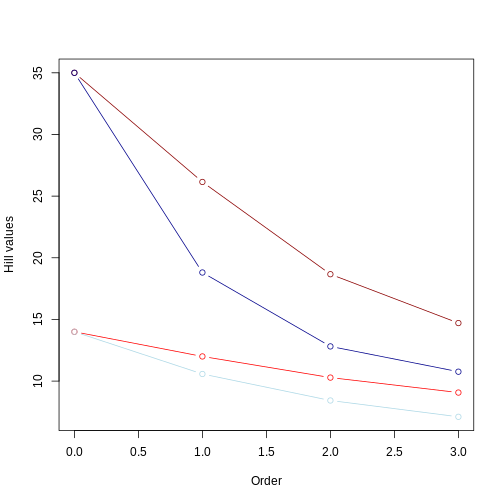
Reminders: 1) light colors represent balanced trees, whereas darker colors represent unbalanced trees 2) red lines represent even community whereas blue lines represent uneven community.
From this second plot, we notice that:
Hill number values for the unbalanced tree (darker colors) are still higher than those for the balanced tree (lighter colors). This makes sense since the relative abundance is the same for both trees, so the overall pattern (i.e., longer branches in unbalanced tree) remains;
the Hill number of order 0 is the same regardless of whether you have different relative abundances among species. This was also the case for example 1. Order 0 is simply the sum of all branch lengths (i.e., it does not account for the relative abundance of branch lengths or taxa);
the inclusion of an uneven community accentuates the rate of decrease in the Hill number value as we increase the order. This is because higher orders are now affected by the unevenness of the distribution of branch length as well by the unevenness of species abundance. This is a good example of how calculating different order of hill numbers while incorporating species abundance allows to have a couple summary statistics accounting for evolutionary history and species abundance distribution that is comparable across different regions.
Keypoints
- The phylogenetic structure of the community (represented by the topology of the tree) influences the evenness of the branch length distribution and contribute to different rates in the decrease of Hill number values as the order number increases.
- The inclusion of community structure (relative abundance of different species) further accentuates this difference in rate of change.
- Phylogenetic Hill numbers represent the sum of branch lenghts. Higher orders weight that sum by the distribution of branch lengths and the species relative abundance.
Now that we acquired an intuition on the information phylogenetic Hill numbers can give us, let’s move on to our actual data.
Moving on to our island communities
For this final section, we will be working on the data for the three island communities to calculate hill numbers from orders of 0 to 3. We will be using our pruned phylogeny and the site-by-species matrix we created in the abundances episode. Since we covered the workflow of calculating phylogenetic Hill numbers in the previous section, we will leave this activity for a challenge.
Challenge
For this challenge, you should calculate the phylogenetic Hill
numbers of orders 0 to 3 for the three islands we are working with
throughout the workshop The key objects here will be the phylogeny
stored in arthro_tree_pruned and the sites-by-species
matrix stored in abundances_wide. You should also plot the
hill numbers for each island and discuss what the calculated values
allow you to infer regarding the history of each community.
We can directly calculate Hill numbers using the
hill_phylo function along with the objects
arthro_tree_pruned and abundances_wide. Since
we have three sites, the function will return a vector with tree values,
one Hill number for each site of the order we requested. Let’s create an
empty list to store a vector for each order, and use a for
loop to calculate from orders of 0 to 3.
R
hill_values <- vector('list', length = 4)
for (i in 0:3) {
    hill_values[[i + 1]] <- hill_phylo(abundances_wide, arthro_tree_pruned,
                                       q = i)
}
Now, let’s create a data.frame with islands as rows and Hill numbers
of different orders as columns. For that, we will use the function
do.call to collapse our list hill_values using
the function cbind.
R
hill_values <- do.call(cbind.data.frame, hill_values)
colnames(hill_values) <- paste0('hill_phylo_', 0:3)
hill_phylo <- data.frame(site = rownames(hill_values),
                         hill_values)

rownames(hill_phylo) <- NULL
hill_phylo
OUTPUT
   site hill_phylo_0 hill_phylo_1 hill_phylo_2 hill_phylo_3
1 BI_01     59.09643     18.71926     13.41881     11.65893
2 MA_01     64.21265     40.30308     26.89875     20.36594
3 KA_01     54.49430     28.10458     20.00878     16.29594
Finally, we can plot using a similar code to the ones we used in our
examples. We set xlim to go from 0 to 3, and
ylim to go from the lowest to the highest value in the
object hill_values. We also add a legend using the
legend() function like we did in the traits episode.
R
plot(seq(0,3),hill_phylo_nbs[3,2:5],
     type='b',col="#440154FF",
     xlab = 'Order',ylab='Hill values',
     xlim = c(0,3),
     ylim = range(min(hill_values),max(hill_values)))
ERROR
Error in eval(expr, envir, enclos): object 'hill_phylo_nbs' not foundR
lines(seq(0,3),hill_phylo_nbs[2,2:5],
      type='b',col="#21908CFF")
ERROR
Error in eval(expr, envir, enclos): object 'hill_phylo_nbs' not foundR
lines(seq(0,3),hill_phylo_nbs[1,2:5],
      type='b',col="#FDE725FF")
ERROR
Error in eval(expr, envir, enclos): object 'hill_phylo_nbs' not foundR
legend(
    "topright",
    legend = c("Kauai","Maui","Big Island"),
    pch = 19,
    col = c("#440154FF", "#21908CFF", "#FDE725FF")
)
ERROR
Error in (function (s, units = "user", cex = NULL, font = NULL, vfont = NULL, : plot.new has not been called yetDiscussion
After calculating and plotting hill numbers, what inferences can you make about the history of these communities, in terms of the rates of local speciation and colonization?
Are there any further visualizations we haven’t done so far that you could make to further investigate the phylogenetic history of each community?
Content from Working with population genetic data
Last updated on 2023-07-11 | Edit this page
Pop gen data
Overview
Questions
- What is genetic diversity?
- What does genetic diversity say about community assembly?
- What are common summaries of genetic diversity within species and communities?
- What are common sequence file formats?
- How do you read in and manipulate sequence data?
- How do you visualize and summarize sequence data?
Objectives
After following this episode, we intend that participants will be able to:
- Understand what genetic diversity is
- Visualize genetic diversity distributions
- Connect genetic diversity distributions to Hill numbers
- Import population genetic data into the R environment
- Manipulate population genetic data
- Calculate genetic diversity \(\pi\)
- Calculate and interpret Hill numbers of genetic diversity
- Interpret amplicon sequence variant data and how it relates to data from gene alignments
Introduction
What is genetic diversity?
GEOBON, in their description of Essential Biodiversity Variables, define intraspecific genetic diversity as:
The variation in DNA sequences among individuals of the same species.
How is this genetic diversity generated? At a proximal level, genetic diversity is generated through the processes of recombination and mutation. These two mechanisms lay the foundation for evolutionary forces like genetic drift, natural selection, and gene flow to shape the distribution of genetic diversity within populations and across communities.
Perhaps one of the most elegant theoretical frameworks for modeling
genetic diversity is coalescent theory. Coalescent theory is a model of
how alleles sampled from a population may have originated from a common
ancestor. Under the assumptions of no recombination, no natural
selection, no gene flow, and no population structure, i.e. neutrality,
it estimates the time to the most recent common ancestor (TMRCA) between
two sampled alleles and the variance of this estimate. When a population
is especially large (i.e. many breeding individuals), the TMRCA of two
randomly sampled alleles is large. This is because the per-generation
probability of two alleles coalescing is 1 / 2Ne, where
Ne, the effective population size, is the number of
breeding individuals in an idealized population that follows the
assumptions stated above. In most, if not all, natural environments
conditions are not ideal and Ne does not perfectly
represent the census size of a population (see Lewontin’s
paradox). While the relationship between Ne and census
population size is not perfect, in most cases Ne increases
as population size increases and can be used to understand the relative
sizes of populations or size changes over time. The intuition is best
understood through visualization.
For a population of 10 diploid individuals (20 allele copies), the probability of two randomly sampled allele coalescing each generation is 1 / (2 * 10), or 1/20. In this single simulation (conducted using Graham Coop’s code) , the two sampled alleles, whose genealogy is traced in blue and red, coalesce 13 generations in the past.
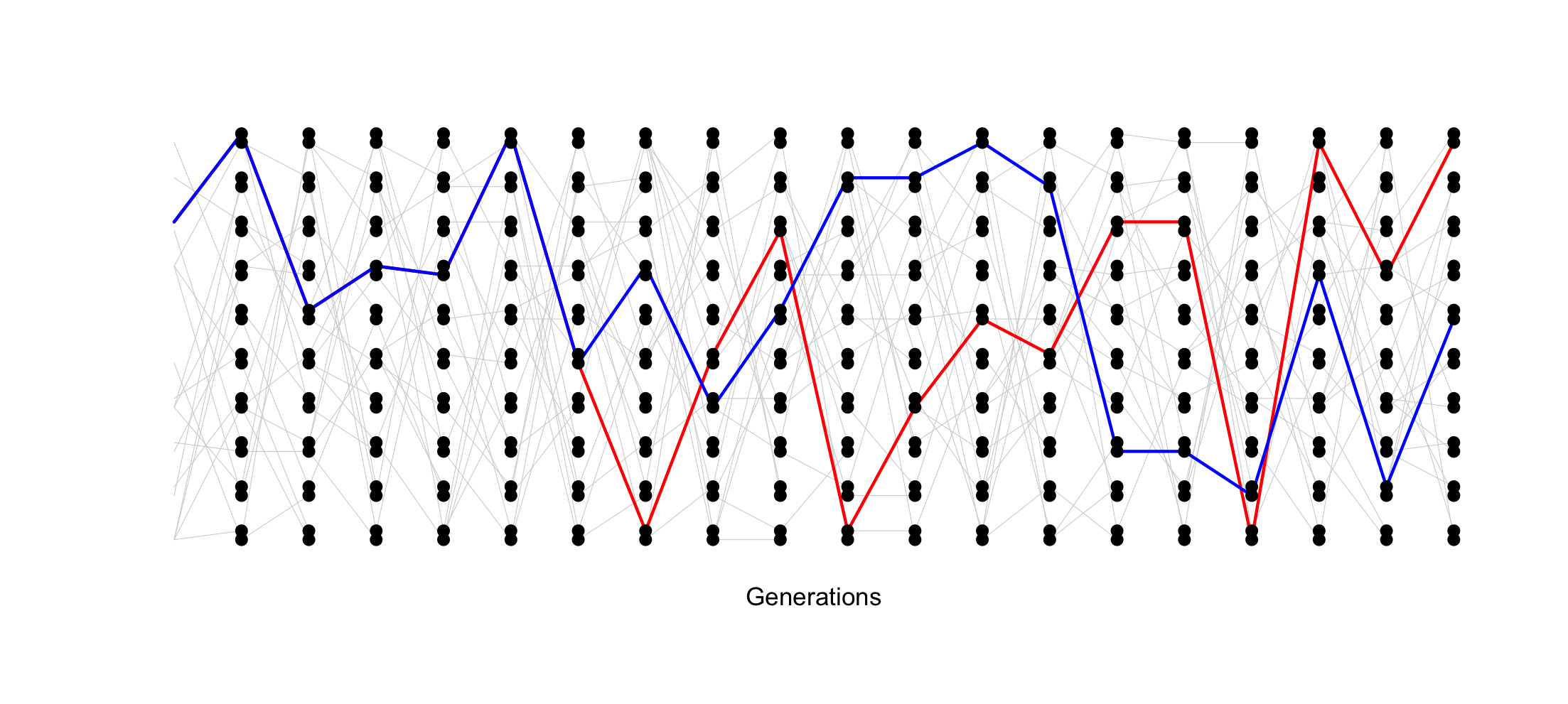
However, when the population is smaller (5 individuals, 10 allele copies), the probability of coalescence each generation is 1 / (2 * 5) or 1/10. In this simulation, two randomly sampled alleles coalesce after 4 generations.
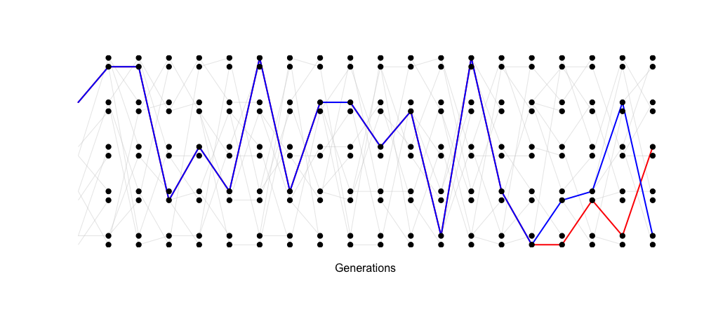
The TMRCA of the two sampled alleles corresponds with the smaller
Ne of this idealized population.
Visualizing this path of ancestry as a tree would look something like this for 5 sampled allele copies.
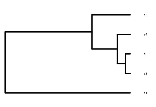
Overlaying mutations on the genealogy results in generally more mutations occurring on longer branches, although because this is a stochastic process, the relationship isn’t always perfect (note- this is a tree from a different simulation to the one above).
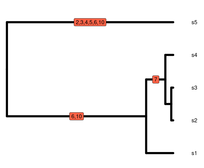
As empirical biologists, what we have to work with are sequence data.
The accumulation of mutations along a sequence enables us to estimate
the TMRCA of a sample of alleles, leading to an estimate of the
Ne of the population.
One of the simplest and most widespread estimators of Ne
is the average number of pairwise differences between sequences sampled
from a population (𝞹, nucleotide diversity, Nei and Li
1979). The basic idea underlying 𝞹 is that more substitutions among
a sample of sequences results from longer branch lengths in the
genealogy of the sample, leading to a longer TMRCA and larger
Ne. The below figure contains the sequence alignment
related to the gene tree beside it. The average number of pairwise
nucleotide differences between s5 and s4 is:
5 (# of nucleotide differences) / 10 (# of basepairs in the sequence) = 0.5
The average number of pairwise nucleotide differences between s4 and s1 is:
1 (# of nucleotide differences) / 10 (# of base pairs in the sequence) = 0.1
The larger number of nucleotide differences between s5 and s4 versus s4 and s1 are reflected in the gene tree, where there the branches are longer leading to the common ancestor of s5 and s4 versus s4 and s1. If we want the genetic diversity of the entire sample of individuals, we add the average pairwise number of nucleotide differences among all of the sequences and take the average of those values.
In this case, \(\pi\) is 0.183!
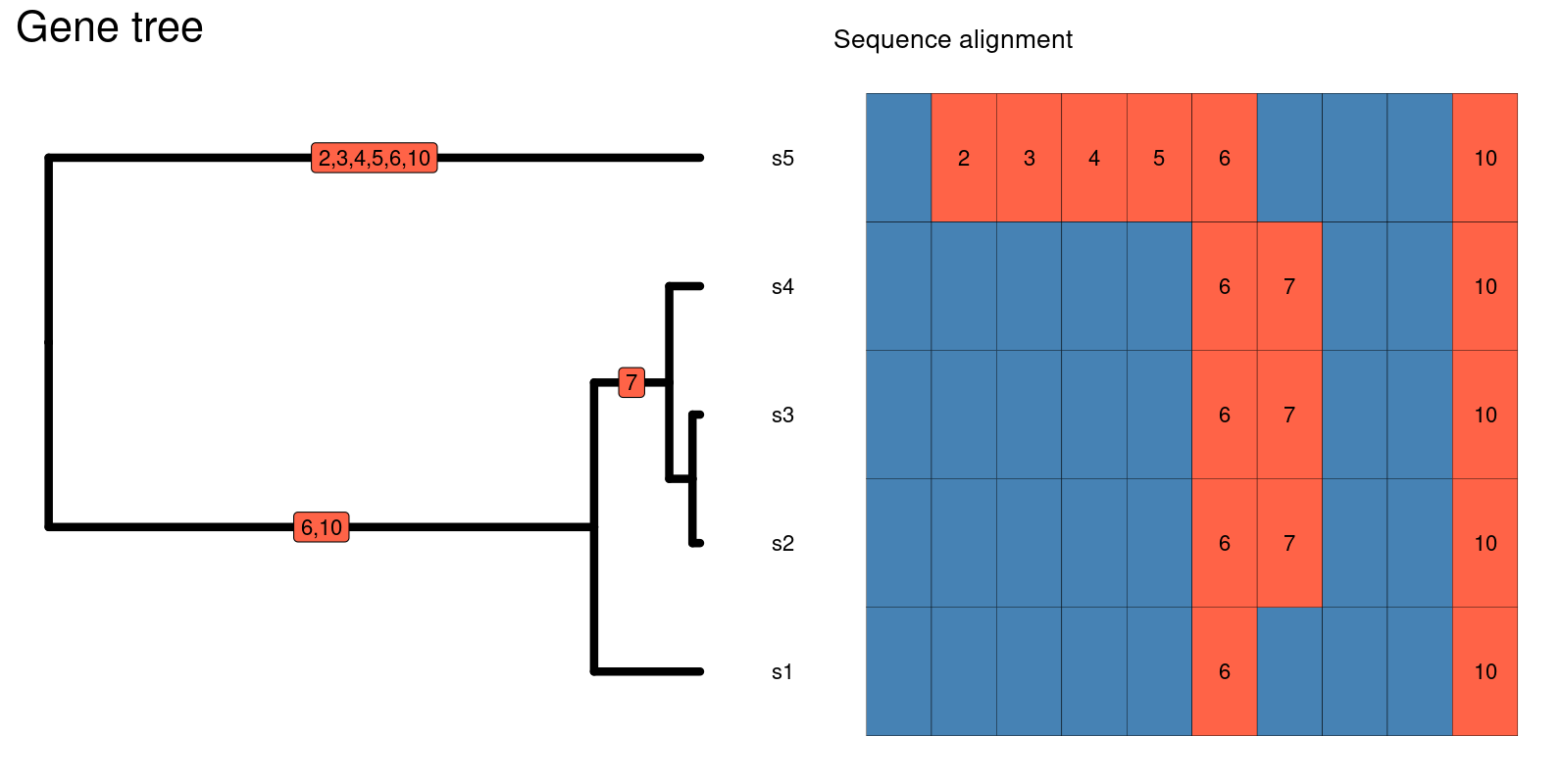
Given its simplicity and ubiquity, we will cover how to calculate the average number of pairwise differences between sequences and summarize this value across assemblages.
Resources for understanding the coalescent
-
- awesome resource for population genetics in general
-
- visualize coalescent genealogies with different numbers of individuals in a population and different numbers of generations
-
- a dynamic and interactive visualization of coalescent genealogies with the ability to change parameters on the fly
-
- a great set of slides that explains the coalescent in a complementary way to Graham Coop’s notes
-
- uses the coalescent to simulate gene trees and mutations along sequences
What does genetic diversity say about community assembly?
Under neutrality and stable demographic histories, variation in genetic diversity across a community reflects differences in long-term population sizes across the community. Rather than a snapshot of present-day abundance, this can be thought of as an average abundance across generations.
In much the same way as a community with a few, highly abundant species and many low abundance species may indicate a non-neutral community assembly process like environmental filtering, a community that contains a few species with high genetic diversity and many species with low genetic diversity may indicate similar non-neutral community assembly processes over a longer timescale.
In addition, genetic diversity is impacted by demographic events and natural selection. Populations that have undergone a demographic expansion or contraction in the recent past will have distinct coalescent genealogies and therefore different genetic diversities. For instance, a population that has experienced a recent demographic expansion will have a TMRCA more recent than a population with the same population size that has remained stable through the same time period, illustrated below.
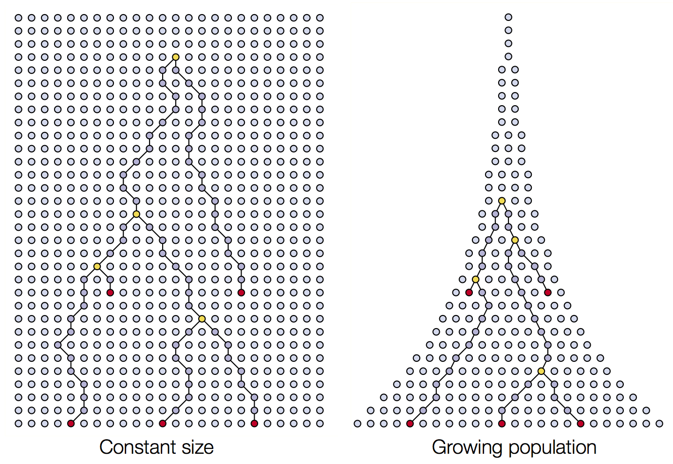
Distinguishing a small, constant-sized population from a large population that’s grown dramatically in the recent past is difficult with single-locus data typical of large-scale biodiversity studies. However, when paired with other data like traits and abundances, we can make more refined interpretations of the shape of genetic diversity across the community. For instance, the interpretation of a community with a few highly diverse species paired with many species with low genetic diversity may reflect a community with a few species that were not impacted by a historical environmental disturbance alongside many species that had their populations dramatically reduced, but have rapidly grown to larger modern population sizes.
Challenge
Draw one or more possible scenarios of a pair of coalescent genealogies drawn from a contracting population. The size of the modern and historical populations and the number of generations you “simulate” are up to you, but you should draw something similar to the figure above.
After completing this exercise, do you think a contracting population would result in more or less genetic diversity?
Contracting populations are funny! If a contraction was recent, the population may maintain the levels of genetic diversity it had before the contraction. However, if the contraction happened in the more distant past and was maintained, genetic diversity is reduced.
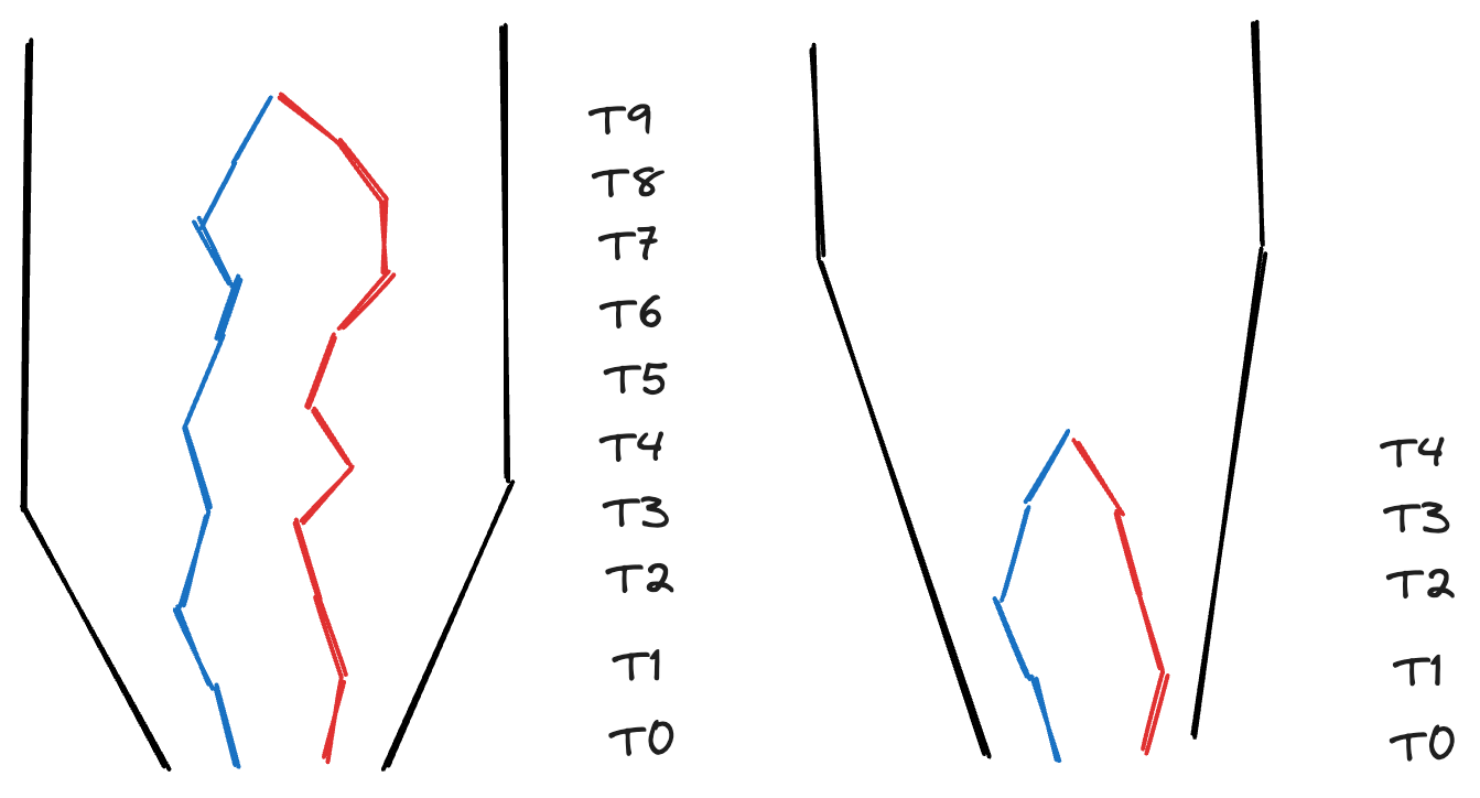
Hill numbers of genetic diversity across species
In the context of summarizing species abundances, Hill numbers are the effective number of species in a community, where each exponent (q-value) increasingly weights common species more heavily. The interpretation is similar when summarizing genetic diversity. Hill numbers are the effective number of species in a community, where each q-value increasingly weights species with higher genetic diversity more heavily. Rather than measuring an effective diversity of abundances, this is an effective diversity of genetic diversities.
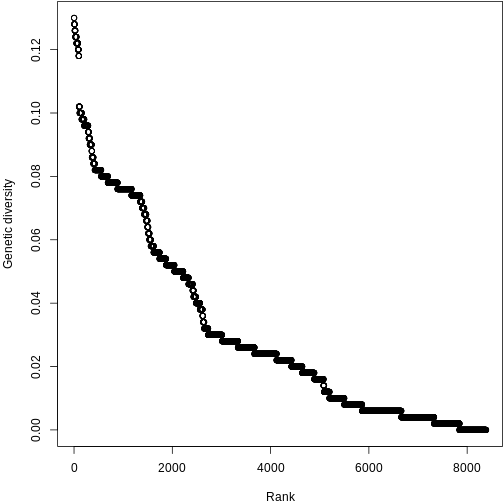
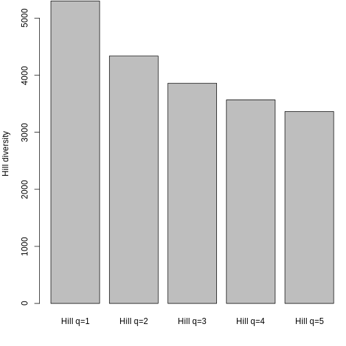
Work with pop gen data
The three packages we’re working with are msa,
ape, and hillR. The first two are used to work
with sequencing data, while hillR is what we will use to
calculate Hill numbers. I’ll provide more explanation once we get to
using them.
R
library(msa)
library(ape)
library(hillR)
Sequences
FASTA
A FASTA file contains one or more DNA sequences, where the DNA sequence is preceded by a line with a carat (“>”) followed by an unique sequence ID:
>seq0010
GATCCCCAATTGGGG
This is perhaps the most common way to store sequence information as it is simple and has historical inertia. For more information, see the the NCBI page.
Alignment
Prior to analysis, sequence data must be aligned if they haven’t been already. A sequence alignment is necessary to identify regions of DNA that are similar or that vary. There are many pieces of software to perform alignments and all have their advantages and disadvantages, but we will choose a single program, Clustal Omega, which is fast and robust for short sequence alignments. While Clustal Omega can be run from the command line, we will use the R package msa to keep everything in the R environment.
First, a FASTA file containing the sequences needs to be read in
using the readDNAStringSet() function. For most of this
episode, we will be working with sequences from the Kauai island. At the
end, we will summarize the
R
seq_path <- "https://raw.githubusercontent.com/role-model/multidim-biodiv-data/main/episodes/data/kauai_seqs.fas"

seqs <- readDNAStringSet(seq_path)

seqs
OUTPUT
DNAStringSet object of length 130:
      width seq                                             names
  [1]   500 CGCGCACTCTACCACCCAGACT...TGACTCCTATCGTTAATTCGTG Proterhinus_punct...
  [2]   500 CGCGCACTCTACCACCCAGACT...TGACTCCTATCGTTAATTCGTG Proterhinus_punct...
  [3]   500 CGCGCACTCTACCACCCAGACT...TGACTCCTATCGTTAATTCGTG Proterhinus_punct...
  [4]   500 CGCGCACTCTACCACCCAGACT...TGACTCCTATCGTTAATTCGTG Proterhinus_punct...
  [5]   500 CGCGCACTCTACCACCCAGACT...TGACTCCTATCGTTAATTCGTG Proterhinus_punct...
  ...   ... ...
[126]   500 CGCGCACTCTACCACCCAGACT...TGACTCCTATCGTTAATTCGTG Campsicnemus_nigr...
[127]   500 CGCGCACTCTACCACCCAGACT...TGACTCCTATCGTTAATTCGTG Campsicnemus_nigr...
[128]   500 CGCGCACTCTACCACCCAGACT...TGACTCCTATCGTTAATTCGTG Campsicnemus_nigr...
[129]   500 CGCGCACTCTACCACCCAGACT...TGACTCCTATCGTTAATTCGTG Campsicnemus_nigr...
[130]   500 CGCGCACTCTACCACCCAGACT...TGACTCCTATCGTTAATTCGTG Campsicnemus_nigr...
To align the sequences using Clustal Omega, we use the
msa function and specify the method as
“ClustalOmega”. There are more arguments that you can use to fine-tune
the alignment, but these are not necessary for the vast majority of
scenarios.
R
alignment <- msa(seqs, method = "ClustalOmega")
OUTPUT
using GonnetR
alignment
OUTPUT
ClustalOmega 1.2.0

Call:
   msa(seqs, method = "ClustalOmega")

MsaDNAMultipleAlignment with 130 rows and 500 columns
      aln                                                  names
  [1] CGCGCACTCTACCACCCAGACTATC...CCGGACTCCTATCGATAATTCGTG Eudonia_lycopodiae-6
  [2] CGCGCACTCTACCACCCAGACTATC...CCCGACTCCTATCGTTAATTCGTG Eudonia_lycopodiae-1
  [3] CGCGCACTCTACCACCCAGACTATC...CCCGACTCCTATCGATAATTCGTG Eudonia_lycopodiae-4
  [4] CGCGCACTCTACCACCCAGACTATC...CCCGACTCCTATCGATAATTCGTG Eudonia_lycopodiae-3
  [5] CGCGCACTCTACCACCCAGACTATC...CCCGACTCCTATCGATAATTCGTG Eudonia_lycopodiae-8
  [6] CGCGCACTCTACCACCCAGACTATC...CCCGACTCCTATCGATAATTCGTG Eudonia_lycopodiae-2
  [7] CGCGCACTCTACCACCCAGACTATC...CCCGACTCCTATCGATAATTCGTG Eudonia_lycopodiae-5
  [8] CGCGCACTCTACCACCCAGACTATC...CCCGACTCCTATCGATAATTCGTG Eudonia_lycopodiae-9
  [9] CGCGCACTCTACCACCCAGACTATC...CCCGACTCCTATCGATAATTCGTG Eudonia_lycopodiae-0
  ... ...
[123] CGCGCACTCTACCACCCAGACTATC...CCTGACTCCTATCGTTAATTCGTG Nesodynerus_mimus-1
[124] CGCGCACTCTACCACCCAGACTATC...CCTGACTCCTATCGTTAATTCGTG Nesodynerus_mimus-5
[125] CGCGCACTCTACCACCCAGACTATC...CCTGACTCCTATCGTTAATTCGTG Nesodynerus_mimus-6
[126] CGCGCACTCTACCACCCAGACTATC...CCTGACTCCTATCGTTAATTCGTG Nesodynerus_mimus-7
[127] CGCGCACTCTACCACCCAGACTATC...CCTGACTCCTATCGTTAATTCGTG Nesodynerus_mimus-0
[128] CGCGCACTCTACCACCCAGACTATC...CCTGACTCCTATCGTTAATTCGTG Nesodynerus_mimus-8
[129] CGCGCACTCTACCACCCAGACTATC...CCTGACTCCTATCGTTAATTCGTG Nesodynerus_mimus-4
[130] CGCGCACTCTACCACCCAGACTATC...CCTGACTCCTATCGTTAATTCGTG Nesodynerus_mimus-9
  Con CGCGCACTCTACCACCCAGACTATC...CCTGACTCCTATCGTTAATTCGTG Consensus
If after you perform your alignment you find that one or more
individuals do not belong or are negatively impacting the alignment, you
have to manipulate your unaligned sequence data and then re-align the
sequences. For instance, say you didn’t want to include the individual
ind_name in the alignment. First, remove the individual
from the seqs object.
R
# remove individual
seqs_filt <- seqs[names(seqs) != "Eudonia_lycopodiae-6"]

seqs_filt
OUTPUT
DNAStringSet object of length 129:
      width seq                                             names
  [1]   500 CGCGCACTCTACCACCCAGACT...TGACTCCTATCGTTAATTCGTG Proterhinus_punct...
  [2]   500 CGCGCACTCTACCACCCAGACT...TGACTCCTATCGTTAATTCGTG Proterhinus_punct...
  [3]   500 CGCGCACTCTACCACCCAGACT...TGACTCCTATCGTTAATTCGTG Proterhinus_punct...
  [4]   500 CGCGCACTCTACCACCCAGACT...TGACTCCTATCGTTAATTCGTG Proterhinus_punct...
  [5]   500 CGCGCACTCTACCACCCAGACT...TGACTCCTATCGTTAATTCGTG Proterhinus_punct...
  ...   ... ...
[125]   500 CGCGCACTCTACCACCCAGACT...TGACTCCTATCGTTAATTCGTG Campsicnemus_nigr...
[126]   500 CGCGCACTCTACCACCCAGACT...TGACTCCTATCGTTAATTCGTG Campsicnemus_nigr...
[127]   500 CGCGCACTCTACCACCCAGACT...TGACTCCTATCGTTAATTCGTG Campsicnemus_nigr...
[128]   500 CGCGCACTCTACCACCCAGACT...TGACTCCTATCGTTAATTCGTG Campsicnemus_nigr...
[129]   500 CGCGCACTCTACCACCCAGACT...TGACTCCTATCGTTAATTCGTG Campsicnemus_nigr...
As a reminder, != means “does not equal”, so
names(seqs) != "Eudonia_lycopodiae-6" returns
TRUE when the sequence name does not match
“Eudonia_lycopodiae-6”.
Following the filtering, you need to realign the new set of sequences.
R
alignment <- msa(seqs_filt, method = "ClustalOmega")
OUTPUT
using GonnetR
alignment
OUTPUT
ClustalOmega 1.2.0

Call:
   msa(seqs_filt, method = "ClustalOmega")

MsaDNAMultipleAlignment with 129 rows and 500 columns
      aln                                                  names
  [1] CGCGCACTCTACCACCCAGACTATC...CCCGACTCCTATCGTTAATTCGTG Eudonia_lycopodiae-1
  [2] CGCGCACTCTACCACCCAGACTATC...CCCGACTCCTATCGATAATTCGTG Eudonia_lycopodiae-4
  [3] CGCGCACTCTACCACCCAGACTATC...CCCGACTCCTATCGATAATTCGTG Eudonia_lycopodiae-3
  [4] CGCGCACTCTACCACCCAGACTATC...CCCGACTCCTATCGATAATTCGTG Eudonia_lycopodiae-8
  [5] CGCGCACTCTACCACCCAGACTATC...CCCGACTCCTATCGATAATTCGTG Eudonia_lycopodiae-2
  [6] CGCGCACTCTACCACCCAGACTATC...CCCGACTCCTATCGATAATTCGTG Eudonia_lycopodiae-5
  [7] CGCGCACTCTACCACCCAGACTATC...CCCGACTCCTATCGATAATTCGTG Eudonia_lycopodiae-9
  [8] CGCGCACTCTACCACCCAGACTATC...CCCGACTCCTATCGATAATTCGTG Eudonia_lycopodiae-0
  [9] CGCGCACTCTACCACCCAGACTATC...CCCGACTCCTATCGATAATTCGTG Eudonia_lycopodiae-7
  ... ...
[122] CGCGCACTCTACCACCCAGACTATC...CCTGACTCCTATCGTTAATTCGTG Nesodynerus_mimus-1
[123] CGCGCACTCTACCACCCAGACTATC...CCTGACTCCTATCGTTAATTCGTG Nesodynerus_mimus-5
[124] CGCGCACTCTACCACCCAGACTATC...CCTGACTCCTATCGTTAATTCGTG Nesodynerus_mimus-6
[125] CGCGCACTCTACCACCCAGACTATC...CCTGACTCCTATCGTTAATTCGTG Nesodynerus_mimus-7
[126] CGCGCACTCTACCACCCAGACTATC...CCTGACTCCTATCGTTAATTCGTG Nesodynerus_mimus-0
[127] CGCGCACTCTACCACCCAGACTATC...CCTGACTCCTATCGTTAATTCGTG Nesodynerus_mimus-8
[128] CGCGCACTCTACCACCCAGACTATC...CCTGACTCCTATCGTTAATTCGTG Nesodynerus_mimus-4
[129] CGCGCACTCTACCACCCAGACTATC...CCTGACTCCTATCGTTAATTCGTG Nesodynerus_mimus-9
  Con CGCGCACTCTACCACCCAGACTATC...CCTGACTCCTATCGTTAATTCGTG Consensus
There are quite a few packages in R to work with sequence data, for
example seqinr,
phangorn,
and ape.
ape is the most versatile of these. But before we can use
ape, the alignment must be converted to the
ape::DNAbin format.
R
ape_align <- msaConvert(alignment, type = "ape::DNAbin")

ape_align
OUTPUT
129 DNA sequences in binary format stored in a matrix.

All sequences of same length: 500

Labels:
Eudonia_lycopodiae-1
Eudonia_lycopodiae-4
Eudonia_lycopodiae-3
Eudonia_lycopodiae-8
Eudonia_lycopodiae-2
Eudonia_lycopodiae-5
...

Base composition:
    a     c     g     t
0.260 0.245 0.234 0.261
(Total: 64.5 kb)
Although not necessary for this workshop (the sequence data is already aligned), it’s generally advisable to write your DNA alignment to a new file to use later or with other programs.
R
ape::write.FASTA(ape_align, "seqs_aligned.fas")
R
# you can also make a vector with the c() function and list each individual separately, but this requires a little less typing
hypo_inds <- paste0("Hyposmocoma_sagittata-", 0:9)

seqs_hypo <- seqs[names(seqs) %in% hypo_inds]

seqs_hypo
OUTPUT
DNAStringSet object of length 10:
     width seq                                              names
 [1]   500 CGCGCACTCTACCACCCAGACTA...TGACTCCTATCGTTAATTCGTG Hyposmocoma_sagit...
 [2]   500 CGCGCACTCTACCACCCAGACTA...TGACTCCTATCGTTAATTCGTG Hyposmocoma_sagit...
 [3]   500 CGCGCACTCTACCACCCAGACTA...TGACTCCTATCGTTAATTCGTG Hyposmocoma_sagit...
 [4]   500 CGCGCACTCTACCACCCAGACTA...TGACTCCTATCGTTAATTCGTG Hyposmocoma_sagit...
 [5]   500 CGCGCACTCTACCACCCAGACTA...TGACTCCTATCGTTAATTCGTG Hyposmocoma_sagit...
 [6]   500 CGCGCACTCTACCACCCAGACTA...TGACTCCTATCGTTAATTCGTG Hyposmocoma_sagit...
 [7]   500 CGCGCACTCTACCACCCAGACTA...TGACTCCTATCGTTAATTCGTG Hyposmocoma_sagit...
 [8]   500 CGCGCACTCTACCACCCAGACTA...TGACTCCTATCGTTAATTCGTG Hyposmocoma_sagit...
 [9]   500 CGCGCACTCTACCACCCAGACTA...TGACTCCTATCGTTAATTCGTG Hyposmocoma_sagit...
[10]   500 CGCGCACTCTACCACCCAGACTA...TGACTCCTATCGTTAATTCGTG Hyposmocoma_sagit...
ape
Check alignment
ape has a useful utility that allows you perform a
series of diagnostics on your alignment to make sure nothing is fishy.
The function can output multiple plots, but let’s just visualize the
alignment plot. If the colors seem jumbled in a region, this indicates
that an alignment error may have occurred and to inspect your sequences
for any problems.
In addition, the function outputs a series of helpful statistics to your console. Ideally, your alignment should have few gaps and a number of segregating sites that is reasonable for the number of sites in your alignment and the evolutionary divergence of the sequences included in the alignment, e.g., for an alignment with 970 sites of a single bird species, around 40 segregating sites is reasonable, but 200 segregating sites may indicate that something went wrong with your alignment or a species was misidentified. In addition, for diploid species a vast majority, if not all of the sites should contain one or two observed bases.
R
checkAlignment(ape_align, what = 1)
OUTPUT
Number of sequences: 129
Number of sites: 500

No gap in alignment.

Number of segregating sites (including gaps): 126
Number of sites with at least one substitution: 126
Number of sites with 1, 2, 3 or 4 observed bases:
  1   2   3   4
374 66 56 4 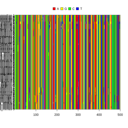
Calculate genetic diversity
To calculate genetic diversity for each species, it’s easiest to
split the alignment by species before calculating the average number of
pairwise nucleotide differences. Since we’re not concerned about
alignment quality, we can just split the alignment, rather than
splitting the original msa sequence object and
re-aligning.
First, you need to get the names of the species. Thankfully, the
genus and species is included in the sequences names, where the format
is “Genus_species-number”. To get the species names, you need to use the
gsub() function, which replaces all of the occurrences of a
particular string pattern in a string. In our case, we need to remove
the “-number” individual identifier at the end of the sequence name, so
we only have “Genus_species”. We will use a short regular expression, or
regex, which is a
sequence of characters that specifies a pattern that a string search
algorithm like gsub() will search for.
The pattern "-[0-9]" means “match any pattern in the
string that is a dash followed by any occurrence of a digit”. The hard
brackets [ ] specify a character set, where any occurrence
of the characters inside the brackets will be matched. In this case, we
specify zero through nine, so any digits that follow a dash will be
matched. The second argument contains the string to replace the pattern
with. We want to remove the pattern, so we supply an empty string to be
replaced.
Following the string removal, we only want unique instances of the
species names, so we use the unique() function to retain
unique species names.
R
sp_names <- gsub("-[0-9]", "", names(seqs))

sp_names <- unique(sp_names)

sp_names
OUTPUT
 [1] "Proterhinus_punctipennis" "Xyletobius_collingei"
 [3] "Metrothorax_deverilli"    "Nesodynerus_mimus"
 [5] "Scaptomyza_vagabunda"     "Lucilia_graphita"
 [7] "Eudonia_lycopodiae"       "Atelothrus_depressus"
 [9] "Mecyclothorax_longulus"   "Laupala_pruna"
[11] "Hylaeus_sphecodoides"     "Hyposmocoma_sagittata"
[13] "Campsicnemus_nigricollis"
Next, we are going to build an R function line-by-line to facilitate creating a list of species alignments. User-defined functions are very useful for when you want to complete a set of tasks repeatedly. Copy-pasting chunks of code and changing things slightly for each situation can lead to errors, headaches, and general pain. The worst bit of pain is when you need to change something in that chunk of code and you have to go back and change it for every instance you copy-pasted it before! When you have a function, you only need to change the code once. I’ll go through each line of code, then we’ll wrap up the code in a function.
First, we need to turn the ape alignment into a list
because the original DNAbin object doesn’t allow
subsetting.
R
align_list <- as.list(ape_align)
The grepl() function searches for a string pattern in
the text, then returns TRUE if it finds it and
FALSE if it doesn’t. We’ll use the resulting boolean
(TRUE/FALSE) vector to extract the species from the
alignment. Here is an example with Proterhinus punctipennis.
You’ll see the 100-110 slots are TRUE, indicating that
those are the locations in the alignment that contain P.
punctipennis sequences.
R
sp_boolean <- grepl("Proterhinus_punctipennis", names(align_list), fixed = TRUE)

sp_boolean
OUTPUT
  [1] FALSE FALSE FALSE FALSE FALSE FALSE FALSE FALSE FALSE FALSE FALSE FALSE
 [13] FALSE FALSE FALSE FALSE FALSE FALSE FALSE FALSE FALSE FALSE FALSE FALSE
 [25] FALSE FALSE FALSE FALSE FALSE FALSE FALSE FALSE FALSE FALSE FALSE FALSE
 [37] FALSE FALSE FALSE FALSE FALSE FALSE FALSE FALSE FALSE FALSE FALSE FALSE
 [49] FALSE FALSE FALSE FALSE FALSE FALSE FALSE FALSE FALSE FALSE FALSE FALSE
 [61] FALSE FALSE FALSE FALSE FALSE FALSE FALSE FALSE FALSE FALSE FALSE FALSE
 [73] FALSE FALSE FALSE FALSE FALSE FALSE FALSE FALSE FALSE FALSE FALSE FALSE
 [85] FALSE FALSE FALSE FALSE FALSE FALSE FALSE FALSE FALSE FALSE FALSE FALSE
 [97] FALSE FALSE FALSE  TRUE  TRUE  TRUE  TRUE  TRUE  TRUE  TRUE  TRUE  TRUE
[109]  TRUE FALSE FALSE FALSE FALSE FALSE FALSE FALSE FALSE FALSE FALSE FALSE
[121] FALSE FALSE FALSE FALSE FALSE FALSE FALSE FALSE FALSE
Following the conversion, we use bracket indexing to subset the
alignment by the sp_boolean boolean vector. Now we have an
alignment of only Proterhinus punctipennis sequences!
R
align_sp <- align_list[sp_boolean]

align_sp
OUTPUT
10 DNA sequences in binary format stored in a list.

All sequences of same length: 500

Labels:
Proterhinus_punctipennis-1
Proterhinus_punctipennis-4
Proterhinus_punctipennis-2
Proterhinus_punctipennis-5
Proterhinus_punctipennis-6
Proterhinus_punctipennis-9
...

Base composition:
    a     c     g     t
0.262 0.242 0.237 0.259
(Total: 5 kb)
Now, we need to wrap these bits of code into a function so we can create separate alignments for all species. The structure of a function looks like this.
R
do_something <- function(x, y) {

}
function() defines the do_something object
as a function, while x and y are the arguments
you are supplying to the function. The curly brackets { }
contain the code you want to run in the function.
For our function split_align, we need two arguments- the
species name we want to extract from the alignment (spname)
and the alignment itself (alignment). We then add our code
inside the curly brackets { }, replacing
"Proterhinus_punctipennis" with spname and
ape_align with alignment. At the end, we
specify that we want to return the align_sp object with the
return() function. Although not always necessary, using the
return() function is generally good practice for code
readability.
R
split_align <- function(spname, alignment) {
    # convert ape object to list
    align_list <- as.list(alignment)

    # get boolean vector for species
    sp_boolean <- grepl(spname, names(align_list), fixed = TRUE)

    # subset alignment for species
    align_sp <- align_list[sp_boolean]

    # return the alignment
    return(align_sp)
}
Now we can check that the function works by running it on Proterhinus punctipennis. It does! (or it should).
R
split_align(spname = "Proterhinus_punctipennis", alignment = ape_align)
OUTPUT
10 DNA sequences in binary format stored in a list.

All sequences of same length: 500

Labels:
Proterhinus_punctipennis-1
Proterhinus_punctipennis-4
Proterhinus_punctipennis-2
Proterhinus_punctipennis-5
Proterhinus_punctipennis-6
Proterhinus_punctipennis-9
...

Base composition:
    a     c     g     t
0.262 0.242 0.237 0.259
(Total: 5 kb)
If your code throws an error or the output isn’t what you expect, you
can place the browser() function at a particular line in
your code to enable you to run it line by line. This helps for
diagnosing where exactly something went wrong.
R
split_align <- function(spname, alignment) {
    browser()
    # convert ape object to list
    align_list <- as.list(alignment)

    # get boolean vector for species
    sp_boolean <- grepl(spname, names(align_list), fixed = TRUE)

    # subset alignment for species
    align_sp <- align_list[sp_boolean]

    # return the alignment
    return(align_sp)
}
Now to apply our function to the vector of species names! We’re using
the lapply() function to apply the split_seqs
function to every element in sp_names and return a list.
lapply() automatically populates the first argument in the
function with the vector or list you supply it, but you can supply
further arguments after entering your function. So, after adding
split_seqs, we specify
alignment = ape_align.
For good measure, we’ll also specify the names of the list elements as the species names, so they’re easy to access later.
R
align_split <- lapply(sp_names, split_align, alignment = ape_align)

names(align_split) <- sp_names

align_split
OUTPUT
$Proterhinus_punctipennis
10 DNA sequences in binary format stored in a list.

All sequences of same length: 500

Labels:
Proterhinus_punctipennis-1
Proterhinus_punctipennis-4
Proterhinus_punctipennis-2
Proterhinus_punctipennis-5
Proterhinus_punctipennis-6
Proterhinus_punctipennis-9
...

Base composition:
    a     c     g     t
0.262 0.242 0.237 0.259
(Total: 5 kb)

$Xyletobius_collingei
10 DNA sequences in binary format stored in a list.

All sequences of same length: 500

Labels:
Xyletobius_collingei-2
Xyletobius_collingei-5
Xyletobius_collingei-0
Xyletobius_collingei-1
Xyletobius_collingei-3
Xyletobius_collingei-4
...

Base composition:
    a     c     g     t
0.262 0.244 0.236 0.259
(Total: 5 kb)

$Metrothorax_deverilli
10 DNA sequences in binary format stored in a list.

All sequences of same length: 500

Labels:
Metrothorax_deverilli-2
Metrothorax_deverilli-8
Metrothorax_deverilli-0
Metrothorax_deverilli-1
Metrothorax_deverilli-3
Metrothorax_deverilli-4
...

Base composition:
    a     c     g     t
0.260 0.246 0.232 0.262
(Total: 5 kb)

$Nesodynerus_mimus
10 DNA sequences in binary format stored in a list.

All sequences of same length: 500

Labels:
Nesodynerus_mimus-2
Nesodynerus_mimus-3
Nesodynerus_mimus-1
Nesodynerus_mimus-5
Nesodynerus_mimus-6
Nesodynerus_mimus-7
...

Base composition:
    a     c     g     t
0.254 0.247 0.237 0.262
(Total: 5 kb)

$Scaptomyza_vagabunda
10 DNA sequences in binary format stored in a list.

All sequences of same length: 500

Labels:
Scaptomyza_vagabunda-4
Scaptomyza_vagabunda-6
Scaptomyza_vagabunda-7
Scaptomyza_vagabunda-8
Scaptomyza_vagabunda-9
Scaptomyza_vagabunda-2
...

Base composition:
    a     c     g     t
0.260 0.247 0.233 0.260
(Total: 5 kb)

$Lucilia_graphita
10 DNA sequences in binary format stored in a list.

All sequences of same length: 500

Labels:
Lucilia_graphita-5
Lucilia_graphita-6
Lucilia_graphita-8
Lucilia_graphita-1
Lucilia_graphita-7
Lucilia_graphita-4
...

Base composition:
    a     c     g     t
0.262 0.240 0.237 0.261
(Total: 5 kb)

$Eudonia_lycopodiae
9 DNA sequences in binary format stored in a list.

All sequences of same length: 500

Labels:
Eudonia_lycopodiae-1
Eudonia_lycopodiae-4
Eudonia_lycopodiae-3
Eudonia_lycopodiae-8
Eudonia_lycopodiae-2
Eudonia_lycopodiae-5
...

Base composition:
    a     c     g     t
0.258 0.248 0.231 0.262
(Total: 4.5 kb)

$Atelothrus_depressus
10 DNA sequences in binary format stored in a list.

All sequences of same length: 500

Labels:
Atelothrus_depressus-0
Atelothrus_depressus-1
Atelothrus_depressus-2
Atelothrus_depressus-3
Atelothrus_depressus-4
Atelothrus_depressus-5
...

Base composition:
    a     c     g     t
0.260 0.246 0.232 0.262
(Total: 5 kb)

$Mecyclothorax_longulus
10 DNA sequences in binary format stored in a list.

All sequences of same length: 500

Labels:
Mecyclothorax_longulus-2
Mecyclothorax_longulus-9
Mecyclothorax_longulus-7
Mecyclothorax_longulus-8
Mecyclothorax_longulus-3
Mecyclothorax_longulus-6
...

Base composition:
    a     c     g     t
0.260 0.244 0.235 0.261
(Total: 5 kb)

$Laupala_pruna
10 DNA sequences in binary format stored in a list.

All sequences of same length: 500

Labels:
Laupala_pruna-1
Laupala_pruna-2
Laupala_pruna-4
Laupala_pruna-8
Laupala_pruna-9
Laupala_pruna-0
...

Base composition:
    a     c     g     t
0.260 0.247 0.233 0.260
(Total: 5 kb)

$Hylaeus_sphecodoides
10 DNA sequences in binary format stored in a list.

All sequences of same length: 500

Labels:
Hylaeus_sphecodoides-7
Hylaeus_sphecodoides-1
Hylaeus_sphecodoides-2
Hylaeus_sphecodoides-3
Hylaeus_sphecodoides-4
Hylaeus_sphecodoides-5
...

Base composition:
    a     c     g     t
0.258 0.248 0.234 0.260
(Total: 5 kb)

$Hyposmocoma_sagittata
10 DNA sequences in binary format stored in a list.

All sequences of same length: 500

Labels:
Hyposmocoma_sagittata-0
Hyposmocoma_sagittata-1
Hyposmocoma_sagittata-2
Hyposmocoma_sagittata-3
Hyposmocoma_sagittata-4
Hyposmocoma_sagittata-5
...

Base composition:
    a     c     g     t
0.260 0.246 0.232 0.262
(Total: 5 kb)

$Campsicnemus_nigricollis
10 DNA sequences in binary format stored in a list.

All sequences of same length: 500

Labels:
Campsicnemus_nigricollis-0
Campsicnemus_nigricollis-1
Campsicnemus_nigricollis-2
Campsicnemus_nigricollis-3
Campsicnemus_nigricollis-4
Campsicnemus_nigricollis-5
...

Base composition:
    a     c     g     t
0.260 0.246 0.232 0.262
(Total: 5 kb)
Now we’re going to calculate the average number of pairwise genetic
differences among these sequences. ape has the
dist.dna() function to calculate various genetic distance
metrics for an alignment.
You use the argument model = "raw" to specify that you
want to use the average number of pairwise differences as your metric.
When calculating the number of pairwise genetic differences, you have to
choose whether you want missing data to be deleted across the entire
alignment (pairwise.deletion = FALSE) or only between the
two sequences being compared (pairwise.deletion = TRUE).
Since we want to take advantage of as much data as possible when
computing 𝜋, we’ll set pairwise.deletion = TRUE.
We’ll do this for a single species, then you’ll get a chance to write your own function to do it across species!
R
fas_gendist <- dist.dna(align_split$Proterhinus_punctipennis, model = "raw", pairwise.deletion = TRUE)

fas_gendist
OUTPUT
                           Proterhinus_punctipennis-1
Proterhinus_punctipennis-4                      0.010
Proterhinus_punctipennis-2                      0.006
Proterhinus_punctipennis-5                      0.006
Proterhinus_punctipennis-6                      0.006
Proterhinus_punctipennis-9                      0.006
Proterhinus_punctipennis-7                      0.008
Proterhinus_punctipennis-0                      0.026
Proterhinus_punctipennis-3                      0.028
Proterhinus_punctipennis-8                      0.024
                           Proterhinus_punctipennis-4
Proterhinus_punctipennis-4
Proterhinus_punctipennis-2                      0.004
Proterhinus_punctipennis-5                      0.004
Proterhinus_punctipennis-6                      0.004
Proterhinus_punctipennis-9                      0.004
Proterhinus_punctipennis-7                      0.006
Proterhinus_punctipennis-0                      0.024
Proterhinus_punctipennis-3                      0.026
Proterhinus_punctipennis-8                      0.022
                           Proterhinus_punctipennis-2
Proterhinus_punctipennis-4
Proterhinus_punctipennis-2
Proterhinus_punctipennis-5                      0.000
Proterhinus_punctipennis-6                      0.000
Proterhinus_punctipennis-9                      0.000
Proterhinus_punctipennis-7                      0.002
Proterhinus_punctipennis-0                      0.020
Proterhinus_punctipennis-3                      0.022
Proterhinus_punctipennis-8                      0.018
                           Proterhinus_punctipennis-5
Proterhinus_punctipennis-4
Proterhinus_punctipennis-2
Proterhinus_punctipennis-5
Proterhinus_punctipennis-6                      0.000
Proterhinus_punctipennis-9                      0.000
Proterhinus_punctipennis-7                      0.002
Proterhinus_punctipennis-0                      0.020
Proterhinus_punctipennis-3                      0.022
Proterhinus_punctipennis-8                      0.018
                           Proterhinus_punctipennis-6
Proterhinus_punctipennis-4
Proterhinus_punctipennis-2
Proterhinus_punctipennis-5
Proterhinus_punctipennis-6
Proterhinus_punctipennis-9                      0.000
Proterhinus_punctipennis-7                      0.002
Proterhinus_punctipennis-0                      0.020
Proterhinus_punctipennis-3                      0.022
Proterhinus_punctipennis-8                      0.018
                           Proterhinus_punctipennis-9
Proterhinus_punctipennis-4
Proterhinus_punctipennis-2
Proterhinus_punctipennis-5
Proterhinus_punctipennis-6
Proterhinus_punctipennis-9
Proterhinus_punctipennis-7                      0.002
Proterhinus_punctipennis-0                      0.020
Proterhinus_punctipennis-3                      0.022
Proterhinus_punctipennis-8                      0.018
                           Proterhinus_punctipennis-7
Proterhinus_punctipennis-4
Proterhinus_punctipennis-2
Proterhinus_punctipennis-5
Proterhinus_punctipennis-6
Proterhinus_punctipennis-9
Proterhinus_punctipennis-7
Proterhinus_punctipennis-0                      0.022
Proterhinus_punctipennis-3                      0.024
Proterhinus_punctipennis-8                      0.020
                           Proterhinus_punctipennis-0
Proterhinus_punctipennis-4
Proterhinus_punctipennis-2
Proterhinus_punctipennis-5
Proterhinus_punctipennis-6
Proterhinus_punctipennis-9
Proterhinus_punctipennis-7
Proterhinus_punctipennis-0
Proterhinus_punctipennis-3                      0.014
Proterhinus_punctipennis-8                      0.010
                           Proterhinus_punctipennis-3
Proterhinus_punctipennis-4
Proterhinus_punctipennis-2
Proterhinus_punctipennis-5
Proterhinus_punctipennis-6
Proterhinus_punctipennis-9
Proterhinus_punctipennis-7
Proterhinus_punctipennis-0
Proterhinus_punctipennis-3
Proterhinus_punctipennis-8                      0.008
The function returns a distance matrix containing the pairwise
differences among all sequences in the data set. To take a quick peak at
their distribution, we can use the hist() function on the
distance matrix.
R
hist(fas_gendist)
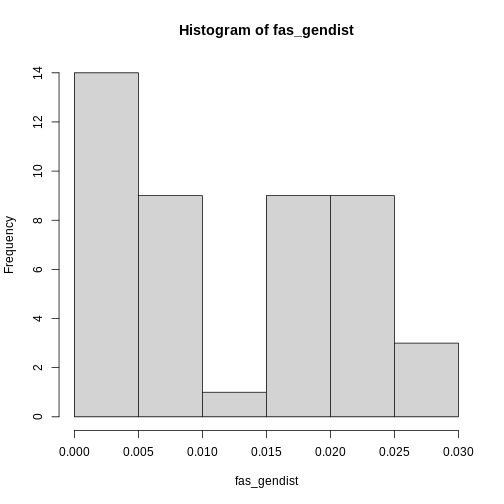
Since we want the average of these differences, we need to take their
average. However, you may have noticed the distribution of genetic
distances is non-normal, with mostly low genetic diversities. This is
the case with most genetic data sets. So, instead of taking the mean,
the median() will provide a better estimate of the center
of the distribution. The average number of pairwise genetic differences,
aka 𝜋, aka genetic diversity of Proterhinus punctipennis is
0.01!
R
fas_gendiv <- median(fas_gendist)

fas_gendiv
OUTPUT
[1] 0.01R
calc_pi <- function(alignment) {
    # get genetic distances
    dists <- dist.dna(alignment, model = "raw", pairwise.deletion = TRUE)
    # get average
    pi <- median(dists)

    return(pi)
}
I haven’t introduced it yet, but sapply() is similar to
lapply(), except it returns a vector instead of a list. It
saves an extra step when you know your function is returning single
values of the same type.
R
# solution 1. This returns a vector
pi_across_sp <- sapply(align_split, calc_pi)

# solution 2
pi_across_sp <- lapply(align_split, calc_pi)
## convert to a vector
pi_across_sp <- unlist(pi_across_sp)
Let’s plot the ranked genetic diversities of Kauai! We’ll use plotting techniques similar to what you’ve used in the Abundance and Traits episodes.
R
plot(sort(pi_across_sp, decreasing = TRUE), xlab = "Rank", ylab = "Genetic diversity")
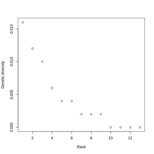
Hill numbers
Now, let’s calculate the first five Hill numbers (q = 1-5) of this
distribution. For this, we will use the hillR package.
hillR does not have a function specifically for calculating
Hill numbers from genetic diversities, but the function you have used
for calculating Hill numbers from abundances, hill_taxa
will work the same.
To turn your vector of genetic diversities into a site by species
matrix, you just need to transpose pi_across_sp with the
t() function. This turns pi_across_sp into a
matrix with a column for each species and a row for each site, which in
this case is 1.
R
pi_t <- t(pi_across_sp)
pi_t
OUTPUT
     Proterhinus_punctipennis Xyletobius_collingei Metrothorax_deverilli
[1,]                     0.01                0.006                 0.002
     Nesodynerus_mimus Scaptomyza_vagabunda Lucilia_graphita Eudonia_lycopodiae
[1,]             0.004                0.004            0.016              0.012
     Atelothrus_depressus Mecyclothorax_longulus Laupala_pruna
[1,]                    0                  0.002         0.002
     Hylaeus_sphecodoides Hyposmocoma_sagittata Campsicnemus_nigricollis
[1,]                    0                     0                        0
Finally, you can feed this matrix into hill_taxa() for
each q value we’re interested in. To make this efficient, let’s use
sapply()!
R
hill_pi <- sapply(1:5, hill_taxa, comm = pi_t)
A quick barplot shows what we expect- Hill decreases with increasing q because it is increasingly weighted by low genetic diversities.
R
barplot(hill_pi, names.arg = c("q=1", "q=2", "q=3", "q=4", "q=5"), ylab = "Hill diversity")
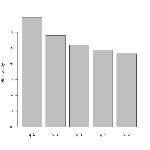
Comparison across islands
Challenge
Lets go through the whole workflow for the Big Island and Maui! Go from the raw sequences to per-species Hill numbers of genetic diversity for both islands. After the challenge we’ll plot genetic diversities and Hill numbers across all three islands and compare!
R
# big island fasta
seqs_bi <- readDNAStringSet("https://raw.githubusercontent.com/role-model/multidim-biodiv-data/main/episodes/data/big_island_seqs.fas")
# maui fasta
seqs_maui <- readDNAStringSet("https://raw.githubusercontent.com/role-model/multidim-biodiv-data/main/episodes/data/maui_seqs.fas")
If you had more islands or localities, you could make a mega-function to get the genetic diversities and/or Hill numbers of each of the localities, rather than copy-pasting this code repeatedly. Functions are very useful!
R
# big island
## align sequences
align_bi <- msa(seqs_bi, method = "ClustalOmega")
OUTPUT
using GonnetR
## convert to DNAbin
ape_align_bi <- msaConvert(align_bi, type = "ape::DNAbin")
## unique names to create alignment list
sp_bi <- unique(gsub("-[0-9]", "", names(seqs_bi)))
## split alignment into list of each species
align_list_bi <- lapply(sp_bi, split_align, alignment = ape_align_bi)
## add names to alignment list
names(align_list_bi) <- sp_bi
## get genetic diversities
pi_bi <- sapply(align_list_bi, calc_pi)
## get Hill numbers 1:5
hill_bi <- sapply(1:5, hill_taxa, comm = t(pi_bi))

# maui
## align sequences
align_maui <- msa(seqs_maui, method = "ClustalOmega")
OUTPUT
using GonnetR
## convert to DNAbin
ape_align_maui <- msaConvert(align_maui, type = "ape::DNAbin")
## unique names to create alignment list
sp_maui <- unique(gsub("-[0-9]", "", names(seqs_maui)))
## split alignment into list of each species
align_list_maui <- lapply(sp_maui, split_align, alignment = ape_align_maui)
## add names to alignment list
names(align_list_maui) <- sp_maui
## get genetic diversities
pi_maui <- sapply(align_list_maui, calc_pi)
## get Hill numbers 1:5
hill_maui <- sapply(1:5, hill_taxa, comm = t(pi_maui))
Now, let’s plot the ranked genetic diversities of each island on the
same plot to compare their shapes. A line plot shows the general shape
of the trend a little clearer, so we’ll set type = "l". We
will use Maui as the base plot, since it has the most species. Then,
we’ll add the other two islands to the plot using the
lines() function.
R
plot(sort(pi_maui, TRUE), type = "l", xlab = "Rank", ylab = "Genetic diversity")
lines(sort(pi_bi, TRUE), col = "red")
lines(sort(pi_across_sp, TRUE), col = "blue")
legend("topright", c("Maui", "Big Island", "Kauai"), fill = c("black", "red", "blue"))
Now, let’s compare Hill q=1 across the three islands. An interesting pattern that we see is that even though Maui has more species, the Hill diversities of the Big Island and Kauai are larger! What is a potential interpretation of these data, especially in light of the abundance and traits data?
R
barplot(c(hill_maui[1], hill_bi[1], hill_pi[1]), names.arg = c("Maui", "Big Island", "Kauai"), ylab = "Hill q=1")
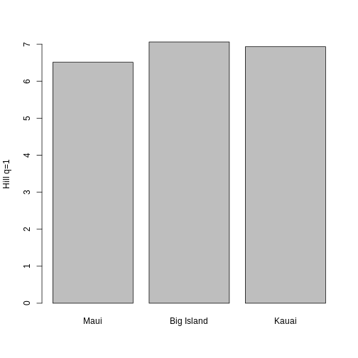
ASVs and Metabarcoding
Metabarcoding is rapidly growing DNA sequencing method used for biodiversity assessment. It involves sequencing a short, variable region of DNA sequence across a sample that may contain many taxa. This can be used to rapidly assess the diversity of a particular sampling site with low sampling effort. Some common applications include microbiome diversity assessments, environmental DNA, and community DNA. In many applications where a data base of species identities for sequence variants is not available or desired, the diversity of sequences is inferred, rather than the diversity of species. Additionally, while there are caveats, the relative abundance of sequences can be considered analogous to the relative abundance of species across a community.
The basic unit of diversity used in most studies is the amplicon sequence variant (ASV). An ASV is any one of the sequences inferred from a high-throughput sequencing experiment. These sequences are free from errors and may diverge by as little as a single base pair from each other. They are considered a substitute for operational taxonomic units (OTUs) for evaluating ecological diversity given their higher resolution, reproducibility, and no need for a reference database.
Sequence table
The basic unit of analysis used for metabarcoding studies is the sequence table. It is a matrix with named rows corresponding to the samples and named columns corresponding to the ASVs. Each cell contains the count of each variant in each sample. Here’s an example with 5 samples and 4 sequence variants:
| asv_1 | asv_2 | asv_3 | asv_4 | |
|---|---|---|---|---|
| sample_1 | 0 | 276 | 200 | 10 |
| sample_2 | 10 | 1009 | 0 | 0 |
| sample_3 | 0 | 0 | 234 | 15 |
| sample_4 | 129 | 1992 | 0 | 485 |
| sample_5 | 1001 | 10 | 1847 | 178 |
sample_1 may correspond to a soil sample collected in a forest, while the variants represent different ASVs, which could look like this:
asv_1: GTTCA
asv_2: GTACA
asv_3: GATCA
asv_4: CTTCA
This looks similiar to a site by species matrix, where the rows are a sampling locality, the columns are the species, and the cell values are the abundance of a species at a particular site.
We’ll briefly go over how the data makes its way from raw sequencing data to the sequence table.
DADA2
DADA2 is one of the most powerful and commonly used software packages for processing raw ASV sequencing data to turn it into a table of ASVs for each sample. This workshop assumes you are using the output from this workflow for further analysis, but for clarity the steps to the workflow include:
- read quality assessment
- filtering and trimming FASTQ files
- learning sequencing error rates, so the algorithm can correct for them
- infer the sequence variants
- merging paired reads (if sequencing was done with forward and reverse read pairs)
- constructing a sequence table
The raw reads are typically in the FASTQ format, which is similar to FASTA, but with some added metadata about the sequences. For more in-depth discussion about FASTQ format, you can scroll to the Extra section!
There are more available to further assess the quality of the data and map the data to taxonomic databases, but the core output of DADA2 and similar software pipelines is the sequence table.
Comparison with sequence alignment workflow
You can analyze ASV data in two ways. You can use the ASV sequencing
table directly and use abundances of each ASV as input into the
hill_taxa() function, considering each ASV as its own
“species”. This has the advantage of using the ASV’s quality as a
minimal reproducible taxonomic unit.
Alternatively, if you have a taxonomic reference database, you can map each ASV to its species identity, convert the table into a FASTA alignment, then calculate metrics like the average number of pairwise nucleotide differences per species. This has the advantage of being able to directly compare genetic diversity metrics with other dimensions of biodiversity like traits and abundances among species. However, the sequence lengths used for ASVs are typically very short and may not capture sufficient variation to characterize species diversity.
Extra
FASTQ
The FASTQ file format is similar to the FASTA format introduced earlier, but includes additional data about the contained sequences. This enables more flexible data manipulation and filtering capabilities, and is popular with high-throughput sequencing technologies. When working with ASVs, this is the most common file format you will encounter.
A FASTA formatted sequence may look like this,
>seq1
GATTTGGGGTTCAAAGCAGTATCGATCAAATAGTAAATCCATTTGTTCAACTCACAGTTT
while a FASTQ version of the same sequence may look like this:
@seq1
GATTTGGGGTTCAAAGCAGTATCGATCAAATAGTAAATCCATTTGTTCAACTCACAGTTT
+
!''*((((***+))%%%++)(%%%%).1***-+*''))**55CCF>>>>>>CCCCCCC65
If your eyes glaze over at the seemingly random numbers below the sequence, don’t fret! They mean something, but usually your machine does the interpreting for you. A FASTQ file is formatted as follows:
An ‘@’ symbol followed by a sequence identifier and an optional description
The raw sequence letters
A ‘+’ character that is optionally followed by the sequence identifier and more description
Quality encodings for the raw sequence letters in field 2. There must be the same number of encoding symbols as there are sequence letters.
The symbols are bytes representing quality, ranging from 0x21 (lowest quality; ‘!’ in ASCII) to 0x7e (highest quality; ‘~’ in ASCII). Here, they’re arranged in order of quality from lowest on the left to highest on the right:
!"#$%&'()*+,-./0123456789:;<=>?@ABCDEFGHIJKLMNOPQRSTUVWXYZ[\]^_`abcdefghijklmnopqrstuvwxyz{|}~Fortunately, whatever bioinformatic program you use will generally do the interpreting for you.
Different sequencing technologies (e.g. Illumina) have standardized description strings which contain more information about the sequences and can be useful when filtering sequences or performing QC. For examples, see the Wikipedia page.
Content from Finding multi-dimensional biodiversity data
Last updated on 2023-07-11 | Edit this page
Overview
Questions
- Where do multi-dimensional biodiversity data live online?
- How can we use R APIs to quickly and reproducibly retrieve data?
- What about data that’s not in a database?
Objectives
After following this episode, we intend that participants will be able to:
- Effectively search for and find occurrence, phylogenetic, sequence, and trait data online given a taxon or research question
- Retrieve data from NCBI & GBIF using their R APIs and apply API principles to other databases
Sources of multidimensional biodiversity data: large open-access databases
Large open-access biological databases have been growing at an incredible pace in recent years. Often they accumulate data from many projects and organizations. These platforms are then used to share and standardize data for wide use.
Many such databases exist, but here are some listed examples:
GBIF contains occurrence records of individuals assembled from dozens of smaller databases.
NCBI (National Center for Biotechnology Information) database, which includes GenBank is the largest repository of genetic data in the world, but includes a lot of biomedical data.
OTOL (Open Tree of Life) is a database that combines numerous published trees and taxonomies into one supertree
GEOME (Genomic Observatories MetaDatabase) contains genetic data associated with specimens or samples from the field.
BOLD (Barcode of Life) is a reference library and database for DNA barcoding
EOL (Encyclopedia of Life) is a species-level platform containing data like taxonomic descriptions, distribution maps, and images
What’s an API?
An API is a set of tools that allows users to interact with a database, such as reading, writing, updating, and deleting data. We can’t go over all of these databases in detail, but let’s cover some examples that illustrate some principles of how these APIs work for different types of biodiversity data.
We can do this using the example of Hawaiian arthropods. Hawaii is known for its diversity of Tetragnatha, a genus of orb weaver spiders. With this target in mind let’s download some occurrence data from GBIF, some sequence data from NCBI, and a phylogeny for Tetragnatha spiders from OTOL.
Using APIs: Setup
For this episode, we’ll be working with some R packages that wrap the APIs of online repositories. Let’s set those up now.
R
library(spocc)
library(rentrez)
library(rotl)
library(taxize)
library(dplyr)
Getting consistent species names using taxize
We will want to source records of the genus Tetragnatha, but
some APIs will require species names rather than the names of broader
taxa like genus or family. We can use the taxize package
for this. taxize links to a genus identification number,
drawn from NCBI, for each genus. We use the get_uid()
function to get this number:
R
uid <- get_uid("Tetragnatha")
Then, we use the downstream() function to get a list of
all species in Tetragnatha.
R
species_uids <- downstream(uid,downto="species")
species_names <- species_uids[[1]]$childtaxa_name

head(species_names)
Occurrence data from GBIF
The spocc package is all about occurrence data and lets
you download occurrences from all major occurrence databases. For GBIF
access using the spocc package, we use the occ()
function.
We’ll put the species names we retrieved as the query
and specify gbif as our target database in the
from field.
Since the occurrences from spocc are organized as a list of
dataframes, one per species, we use the bind_rows()
function from dplyr to combine this into a single
dataframe.
We can also specify a geographic bounding box of where we’d like to look for occurrences. Here we’re using a bounding box that covers the Hawaiian Islands.
R
occurrences <- occ(query = species_names, from = 'gbif', has_coords=TRUE,
                   gbifopts=list("decimalLatitude"='18.910361,28.402123',
                                 "decimalLongitude"='-178.334698,-154.806773'))

# extract the data from gbif
occurrences_gbif <- occurrences$gbif$data

# the results in `$data` are a list with one element per species,
# so we combine all those elements
occurrences_df <- bind_rows(occurrences_gbif)

# plot coordinates of occurrences colored by species
plot(occurrences_df$longitude,occurrences_df$latitude,
     cex=0.25,ylab="Latitude",xlab="Longitude",
     col=as.factor(occurrences_df$species))
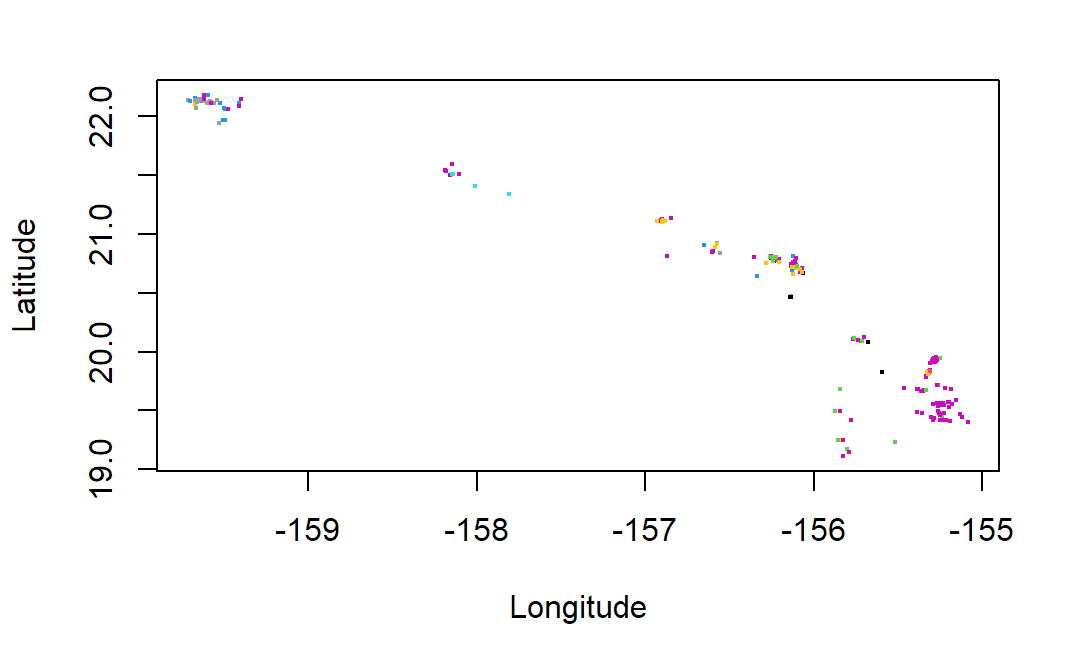
The occ() function returned an object of class occDat. It contains members for each database you could have queried, like “gbif” or “ebird”. Each of these members contains members called “data” which holds the actual data, and “meta” which contains metadata on what we searched for and how it was returned. The “data” object is a list where each member of the list holds a dataframe of records for a different species. As described we can use “bind_rows” from dplyr to create a composite dataframe from this list.
But wait, what is occurrence data?
Occurrence is related to abundance in that it also describes how species are distributed in space but is different in some important ways.
A single abundance data point describes the amount of individuals of a species in a certain area.
But a single occurrence data point describes the presence of a SINGLE individual in a location.
Occurrence data is vastly more common than abundance data online, but often comes with much greater bias in the way it captures the distribution of biodiversity. It is often “incidental”. A citizen scientist happening to record a new butterfly they saw on their morning hike (occurrence) or a researcher electing to record a rare beetle they were looking for (occurrence) are much less systematic and more biased than the field surveys specifically intended to monitor abundance.
Due to this bias it is often used just to indicate presence-absence of a species rather than the magnitude of its population size.
It can be possible to obtain “abundance-like” information from occurrences, but it requires VERY careful consideration of bias and uncertainty.
Phylogenetic trees from the Open Tree of Life
First we’ll get a clean list of taxonomic names from the GBIF
results. We could use our initial names we got from taxize,
but using our GBIF results conveniently narrows things down to Hawaii
species only.
R
species_names_hawaii <- unique(occurrences_df$name)
species_names_resolved <- gnr_resolve(species_names_hawaii, best_match_only = TRUE,
                          canonical = TRUE)
species_names_hawaii <- species_names_resolved$matched_name2
Now we can use the rotl package. The rotl
package provides an interface to the Open Tree of Life. To get a tree
from this database, we have to match our species names to OTOL’s
ids.
We first use trns_match_names() to match our species
names to OTOL’s taxonomy.
Then we use ott_id() to get OTOL ids for these matched
names.
R
species_names_otol <- tnrs_match_names(species_names_hawaii)
otol_ids <- ott_id(species_names_otol)
Finally, we get the tree containing these IDs as tips.
R
tr <- tol_induced_subtree(ott_ids = otol_ids)
plot(tr)
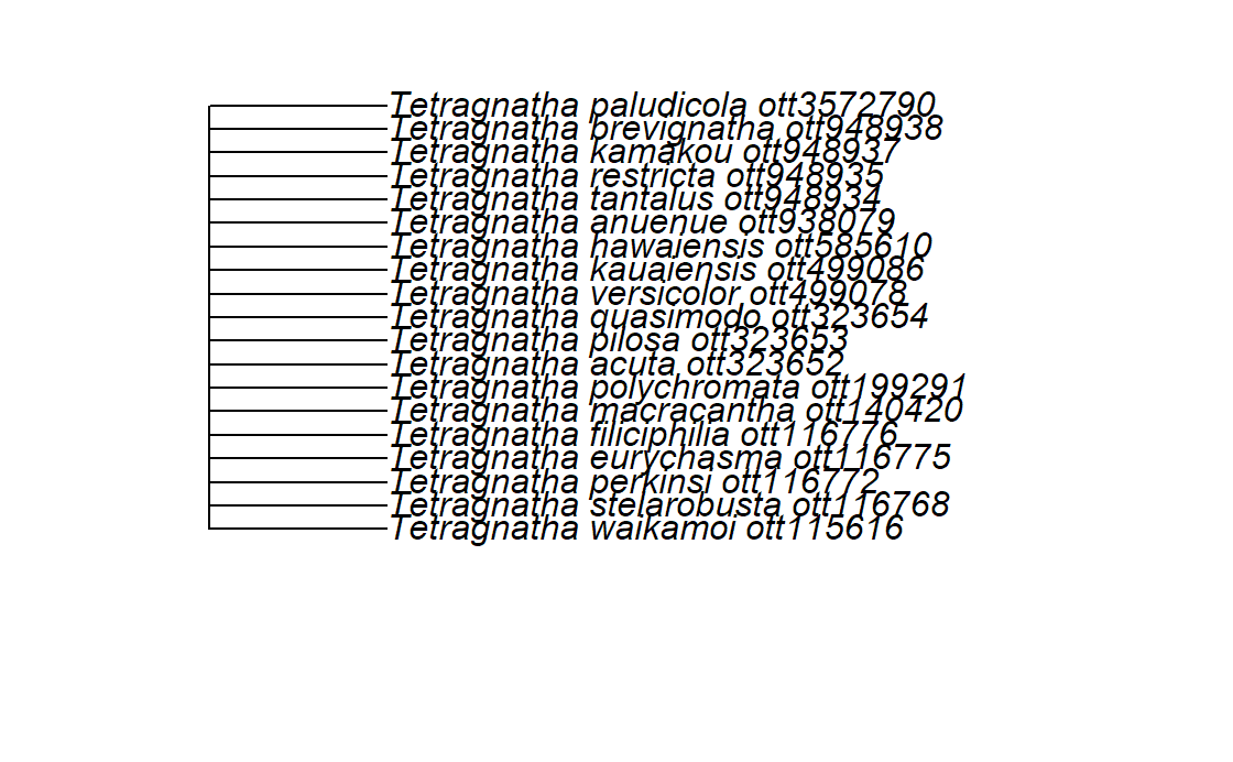
Unfortunately we can see that the phylogenetic relationships between these species aren’t resolved in OTOL, so we may have to look elsewhere for a phylogeny. This is an example of how not all the data we are looking for are in large repositories, especially higher resolution phylogenies.
Sequence data from NCBI
Let’s continue with the rentrez package, which provides
an interface to NCBI. The two usual steps for querying from NCBI is an
ID search using entrez_search() and a records fetch using those IDs in
entrez_fetch(). Sound a bit familiar?
We’ll again search for the species in our Hawaii occurrences.
The main arguments of the entrez_search() function are “db”, the database to look in, and “term” a string representing the whole query. While the occ() function had multiple fields for different ways we are narrowing our search, the “term” field wraps this up in a single string.
R
# we're using `species_names` that we made previously to make a long
# string of names that will be sent to NCBI via the ENTREZ API
termstring <- paste(sprintf('%s[ORGN]', species_names_hawaii), collapse = ' OR ')

search_results <- entrez_search(db="nucleotide", term = termstring)

# take a quick look at all the possible things we could have added to term for this database - it includes [GENE] for looking for specific genes or [SLEN] for length of sequence
entrez_db_searchable(db="nucleotide")
Unlike spocc but similarly to
rotl, this first search returns a set of IDs.
We then have to use entrez_fetch() on the IDs in
search_results to obtain the actual record information.
We specify ‘db’ as ‘nucleotide’ and ‘rettype’ as ‘fasta’ to get FASTA sequences
R
sequences <- entrez_fetch(db = "nucleotide", id = search_results$ids,
                          rettype = "fasta")

# just look at the first part of this *long* returned string
# substr gets characters 1 through 1148 of the FASTA, and cat simply prints it with line breaks
cat(substr(sequences,1,1148))
NCBI and OTOL both require an initial search to obtain record IDs, then a second fetch to obtain the actual record data for each ID
NCBI uses a string-based query where the search is a specially-formated string, while GBIF uses an argument-based query where the search is based on the various arguments you give to the R function.
NCBI is capable of taking a genus and returning the records of all its species, but OTOL and GBIF require obtaining the species names first using a package like taxize
GBIF data is formatted as a list of occurrences for each species contained in the object we get from the query.
Sources of MDBD: Databases without APIs
Many excellent databases exist without specialized APIs or R packages to facilitate their use.
For example, the BioTIME database is a compilation of timeseries of species ocurrence, abundance, and biomass data. It is openly available via the University of St. Andrews. The North American Breeding Bird Survey, run by the USGS, contains data on bird species abundances across the United States and Canada going back more than 50 years. These data are hosted on ScienceBase.
Some of these databases can be accessed via the Data Retriever and
accompanying R package the rdataretriever.
Some are findable via DataONE and the Ecological Data Initiative.
Others can be downloaded directly from the source.
Sources of MDBD: “small data” attached to papers
Finally, A lot of useful data is not held in databases, and is instead attached to papers. Searching manuscript databases or Google Scholar can be an effective way to find such data. You can filter Web of Science to find entries with “associated data”.
However, this can still be a somewhat heterogeneous and time-consuming strategy!
Recap
Keypoints
- Many sources exist online where multidimensional biodiversity data can be obtained
- APIs allow for fast and reproducible querying and downloading
- While there are patterns in how these APIs work, there will always be differences between databases that make using each API a bit different.
- Standalone databases and even the supplemental data in manuscripts can also be re-used.
Content from CARE Principles and Data Repositories
Last updated on 2023-07-11 | Edit this page
Overview
Questions
- What biodiversity data repositories implement CARE principles?
- How can we use the Local Contexts Hub API to link data records with Indigenous data provenance and rights?
Objectives
After following this episode, participants should be able to…
- Articulate the challenges to implementing CARE in biodiversity data sharing
- Use the Local Contexts Hub API to retrieve TK/BC Labels and Notices
What biodiversity repositories utilize TK/BC Labels and Notices?
Not much! Here are two: - GEOME - Maine-eDNA database
Are existing metadata standards sufficient for housing information about Indigenous data sovereignty and governance?
Challenge
- Look up the descriptions of Biocultural Labels and Notices
- Look up the fields of the Darwin Core metadata standard
- Can they interoperate?
There is no agreed upon solution. So the solution is really more of a conversation at this point. One key concept to keep in mind is that Darwin Core (and other metadata standards) are built upon a settler system of data management, data provenance, and intellectual property. That system was created to manifest the rights of settlers and to destroy the rights of Indigenous people, communities, and peoples. So perhaps the terms can be translated, but perhaps this will not be satisfactory without rebuiling standards with both CARE and FAIR principles at heart.
What can we do without institutional support from large repositories (yet)?
The Local Contexts Hub provides an API that we can use in our data workflows to ensure that Indigenous data sovereignty metadata propagate along with the data.
Let’s see how we can use the Local Contexts Hub API to query information about the Maine-eDNA project we learned about. We can find the API documentation here.
R
library(jsonlite)
library(httr)

# the API documentation tells us this is the base URL to access the API
baseURL <- "https://localcontextshub.org/api/v1"

# to retrive project information, we add this to the base URL
projDetail <- "/projects/<PROJECT_UNIQUE_ID>/"

# we need to know the protect ID, we can find it in our LC Hub account
projID <- "6d34be51-0f60-4fc5-a699-bed4091c02e0"

# now we start to construct our query string
q <- paste0(baseURL, projDetail)
q
OUTPUT
[1] "https://localcontextshub.org/api/v1/projects/<PROJECT_UNIQUE_ID>/"R
# we need to replace "<PROJECT_UNIQUE_ID>" with `projID`
q <- gsub("<PROJECT_UNIQUE_ID>", projID, q)
q
OUTPUT
[1] "https://localcontextshub.org/api/v1/projects/6d34be51-0f60-4fc5-a699-bed4091c02e0/"R
# now we can use functions from jsonlite and httr to pull the info
rawRes <- GET(q)
jsonRes <- rawToChar(rawRes$content)

res <- fromJSON(jsonRes)

# have a look
res
OUTPUT
$unique_id
[1] "6d34be51-0f60-4fc5-a699-bed4091c02e0"

$providers_id
NULL

$source_project_uuid
NULL

$project_page
[1] "https://localcontextshub.org/projects/6d34be51-0f60-4fc5-a699-bed4091c02e0/"

$title
[1] "Maine-eDNA Index Sites"

$project_privacy
[1] "Public"

$date_added
[1] "2022-06-03T14:31:52.076304Z"

$date_modified
[1] "2022-07-19T22:46:07.421725Z"

$created_by
  institution.id                 institution.institution_name researcher
1             44 Maine Center for Genetics in the Environment         NA
  community
1        NA

$notice
  notice_type                    name
1 biocultural Biocultural (BC) Notice
                                                                                                img_url
1 https://storage.googleapis.com/anth-ja77-local-contexts-8985.appspot.com/labels/notices/bc-notice.png
                                                                                                svg_url
1 https://storage.googleapis.com/anth-ja77-local-contexts-8985.appspot.com/labels/notices/bc-notice.svg
                                                                                                                                                                                                                                                                                                                                                                                                                                                                                                                                                                                      default_text
1 The BC (Biocultural) Notice is a visible notification that there are accompanying cultural rights and responsibilities that need further attention for any future sharing and use of this material or data. The BC Notice recognizes the rights of Indigenous peoples to permission the use of information, collections, data and digital sequence information (DSI) generated from the biodiversity or genetic resources associated with traditional lands, waters, and territories. The BC Notice may indicate that BC Labels are in development and their implementation is being negotiated.
                      created                     updated
1 2022-06-03T14:31:52.433462Z 2022-07-19T21:37:44.711129Z

$sub_projects
list()

$related_projects
list()

$project_boundary_geojson
NULL
There’s a lot of info there! If a Notice is attached to the project,
we can access it directly with res$notice. Similarly, if TK
and/or BC labels are associated with the project they can be accessed
with res$tk_labels and res$bc_labels,
respectively.
There is an R package enRich under development by Jacob Golan in collaboration with ENRICH that can wrap these API calls in more familiar-looking R code. We have to install this in-dev package from github:
R
remotes::install_github("jacobgolan/enRich")
library(enRich)
Now we can re-produce the previous API call in simpler R code
R
projID <- "6d34be51-0f60-4fc5-a699-bed4091c02e0"
meDNA <- find.projects(projID)
meDNA
The idea of pulling information from Local Contexts Hub via the API is that, for example, reports and manuscripts can now use calls to the API to automatically disclose Indigenous rights and interests in the data underlying the data used.
As an example, a manuscript written using RMarkdown or Quarto could include the following in the introduction
MARKDOWN
```{r LCH-setup}
projID <- "259854f7-b261-4c8c-8556-4b153deebc18"
thisProj <- find.projects(projID)

comms <- thisProj[[1]]$bc_labels$community
```

We make use of data originating from `comms` traditional territories.
These data thus have `comms` provenance, in spite of any settler concept
of data ownership. To affirm the intrinsic rights of `comms` communities
to govern the collection, use, and sharing of their data, `comms`
applied the following Biocultural Labels to these data, specifying
ethical protocol for the use and management of these data:

```{r bc-labels, results = 'asis'}
allBCLabels <- thisProj[[1]]$bc_labels

for(i in 1:length(allBCLabels)) {
    thisLab <- allBCLabels$label_text[i]

    cat(thisLab, "\n")
}
```
This code will render the community name and BC Labels they have applied.
As researchers we can also host our data outside of large online repositories, but still have them FAIR and CARE using webhooks to query the Local Contexts API. This is the approach taken by the Maine-eDNA database infrastructure.
For the purpose of sharing data with Indigenous sovereignty metadata, enRich also provides an experimental method for attaching Local Contexts Hub IDs to sequence data.
R
# read in a fasta file using the dedicated function from enRich
seqs <- readFASTA('https://raw.githubusercontent.com/role-model/multidim-biodiv-data/main/episodes/data/big_island_seqs.fas')

# just for demonstration purposes, set up a temporary directory
temp <- tempdir()

# write out the file
outputFASTA(
    seqs = seqs$sequence,
    seqid = seqs$name,
    uqID = projID, # the uniqe ID for the project we found above in Step 3
    filename = file.path(temp, "seqs-LCH-ID") # .fasta is automatically added
)

# read it back in and notice that the LC Hub ID is now in the fasta header
res <- readLines(file.path(temp, "seqs-LCH-ID.fasta"), n = 10)
cat(res)
This approach could be taken before uploading sequence data to GenBank.