Working with population genetic data
Last updated on 2023-07-11 | Edit this page
Pop gen data
Overview
Questions
- What is genetic diversity?
- What does genetic diversity say about community assembly?
- What are common summaries of genetic diversity within species and communities?
- What are common sequence file formats?
- How do you read in and manipulate sequence data?
- How do you visualize and summarize sequence data?
Objectives
After following this episode, we intend that participants will be able to:
- Understand what genetic diversity is
- Visualize genetic diversity distributions
- Connect genetic diversity distributions to Hill numbers
- Import population genetic data into the R environment
- Manipulate population genetic data
- Calculate genetic diversity \(\pi\)
- Calculate and interpret Hill numbers of genetic diversity
- Interpret amplicon sequence variant data and how it relates to data from gene alignments
Introduction
What is genetic diversity?
GEOBON, in their description of Essential Biodiversity Variables, define intraspecific genetic diversity as:
The variation in DNA sequences among individuals of the same species.
How is this genetic diversity generated? At a proximal level, genetic diversity is generated through the processes of recombination and mutation. These two mechanisms lay the foundation for evolutionary forces like genetic drift, natural selection, and gene flow to shape the distribution of genetic diversity within populations and across communities.
Perhaps one of the most elegant theoretical frameworks for modeling
genetic diversity is coalescent theory. Coalescent theory is a model of
how alleles sampled from a population may have originated from a common
ancestor. Under the assumptions of no recombination, no natural
selection, no gene flow, and no population structure, i.e. neutrality,
it estimates the time to the most recent common ancestor (TMRCA) between
two sampled alleles and the variance of this estimate. When a population
is especially large (i.e. many breeding individuals), the TMRCA of two
randomly sampled alleles is large. This is because the per-generation
probability of two alleles coalescing is 1 / 2Ne, where
Ne, the effective population size, is the number of
breeding individuals in an idealized population that follows the
assumptions stated above. In most, if not all, natural environments
conditions are not ideal and Ne does not perfectly
represent the census size of a population (see Lewontin’s
paradox). While the relationship between Ne and census
population size is not perfect, in most cases Ne increases
as population size increases and can be used to understand the relative
sizes of populations or size changes over time. The intuition is best
understood through visualization.
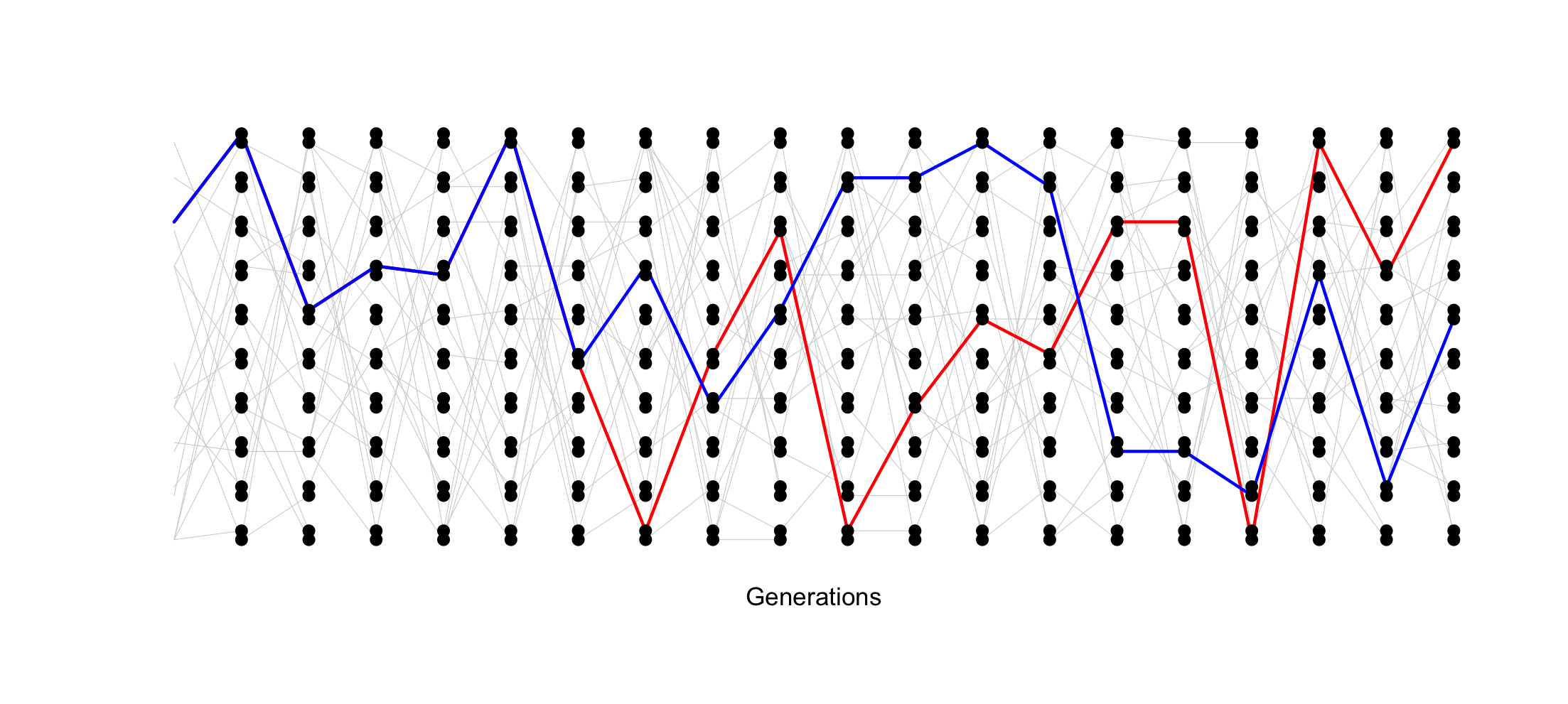
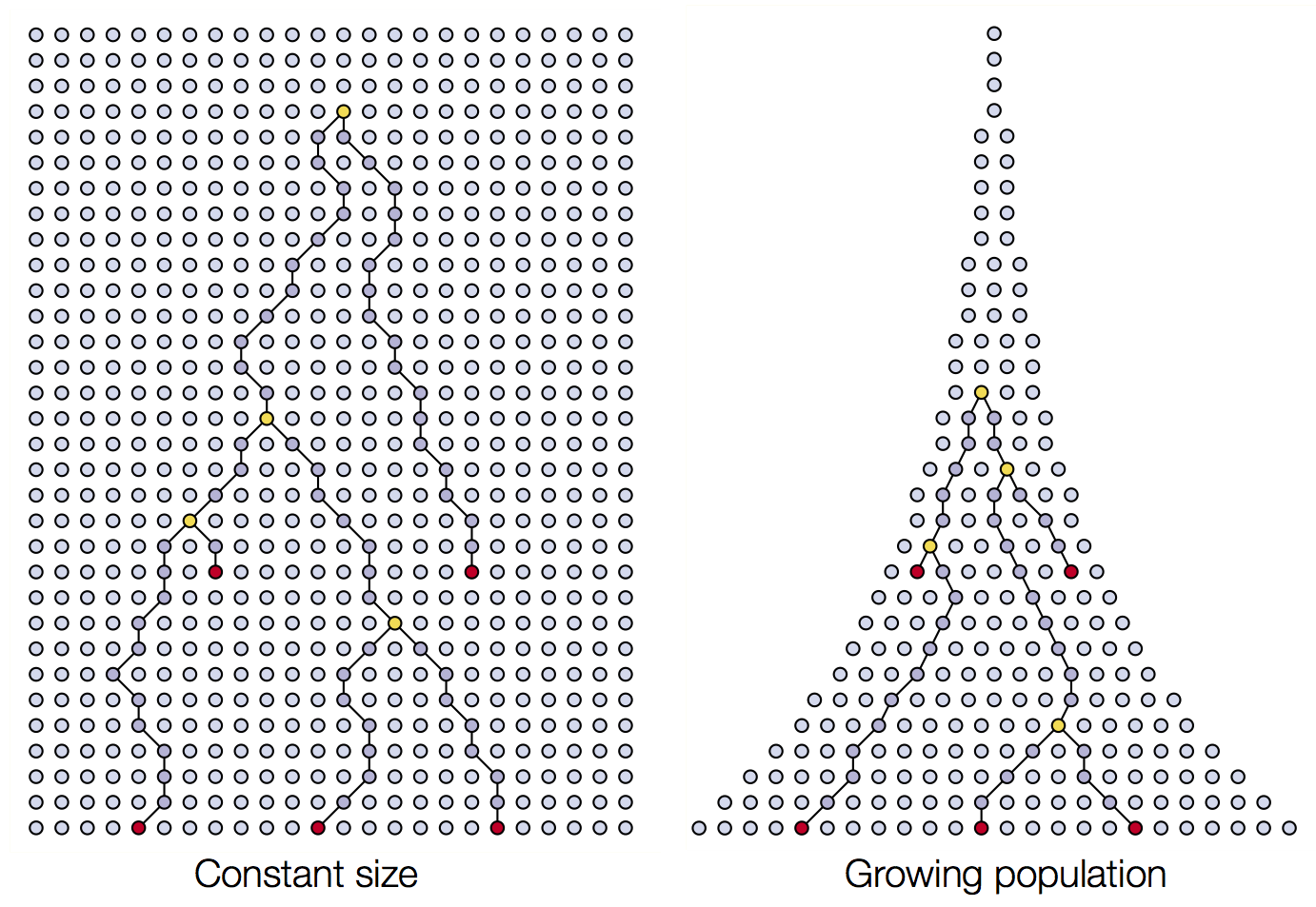
For a population of 10 diploid individuals (20 allele copies), the probability of two randomly sampled allele coalescing each generation is 1 / (2 * 10), or 1/20. In this single simulation (conducted using Graham Coop’s code) , the two sampled alleles, whose genealogy is traced in blue and red, coalesce 13 generations in the past.
However, when the population is smaller (5 individuals, 10 allele copies), the probability of coalescence each generation is 1 / (2 * 5) or 1/10. In this simulation, two randomly sampled alleles coalesce after 4 generations.
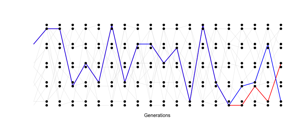
The TMRCA of the two sampled alleles corresponds with the smaller
Ne of this idealized population.
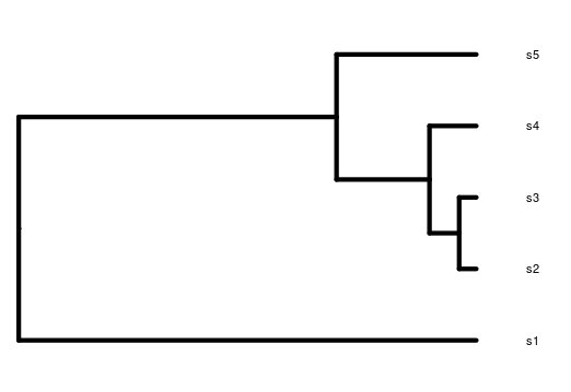
Visualizing this path of ancestry as a tree would look something like this for 5 sampled allele copies.
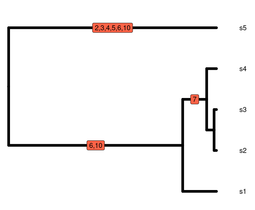
Overlaying mutations on the genealogy results in generally more mutations occurring on longer branches, although because this is a stochastic process, the relationship isn’t always perfect (note- this is a tree from a different simulation to the one above).
As empirical biologists, what we have to work with are sequence data.
The accumulation of mutations along a sequence enables us to estimate
the TMRCA of a sample of alleles, leading to an estimate of the
Ne of the population.
One of the simplest and most widespread estimators of Ne
is the average number of pairwise differences between sequences sampled
from a population (𝞹, nucleotide diversity, Nei and Li
1979). The basic idea underlying 𝞹 is that more substitutions among
a sample of sequences results from longer branch lengths in the
genealogy of the sample, leading to a longer TMRCA and larger
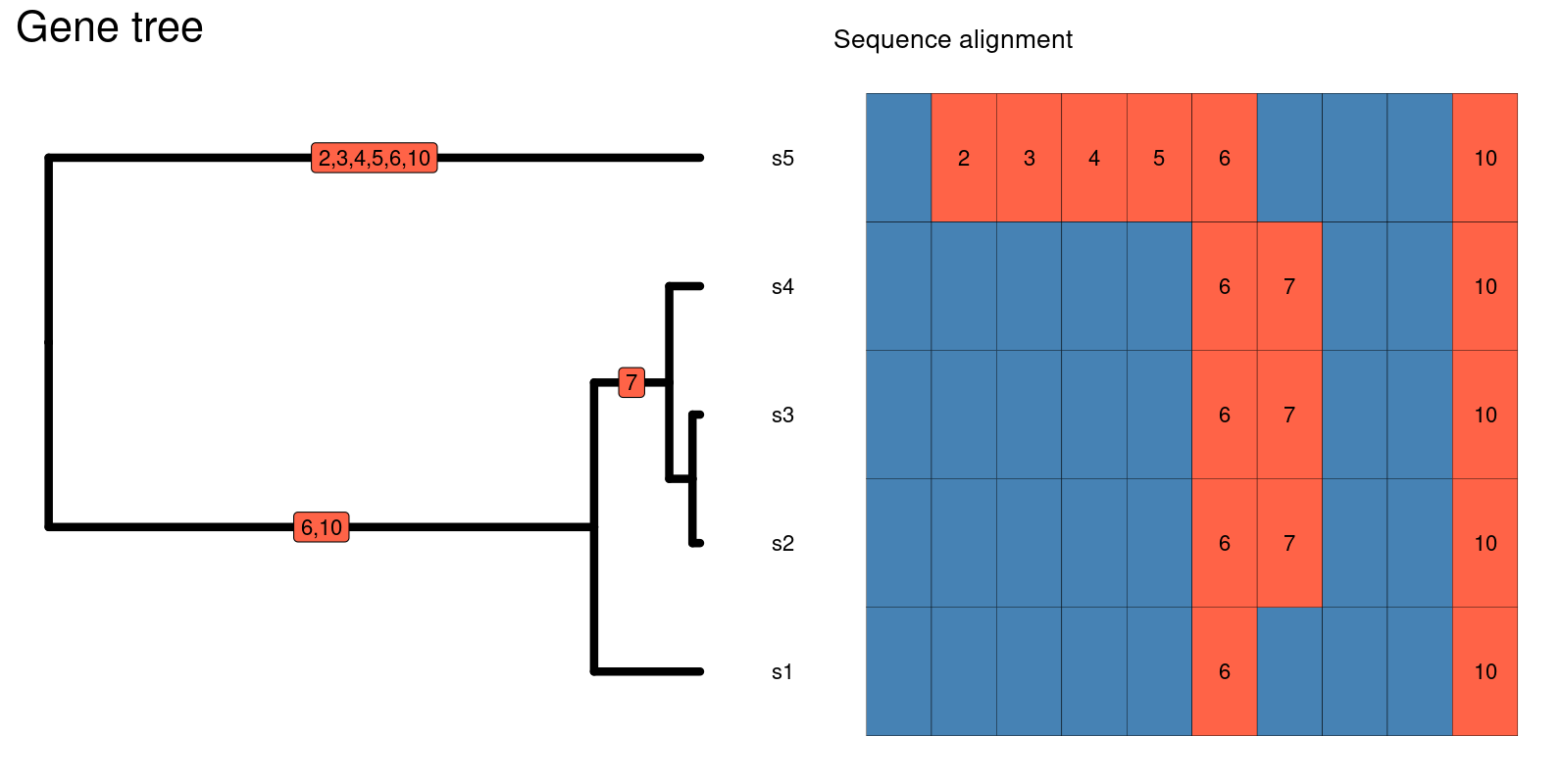
Ne. The below figure contains the sequence alignment
related to the gene tree beside it. The average number of pairwise
nucleotide differences between s5 and s4 is:
5 (# of nucleotide differences) / 10 (# of basepairs in the sequence) = 0.5
The average number of pairwise nucleotide differences between s4 and s1 is:
1 (# of nucleotide differences) / 10 (# of base pairs in the sequence) = 0.1
The larger number of nucleotide differences between s5 and s4 versus s4 and s1 are reflected in the gene tree, where there the branches are longer leading to the common ancestor of s5 and s4 versus s4 and s1. If we want the genetic diversity of the entire sample of individuals, we add the average pairwise number of nucleotide differences among all of the sequences and take the average of those values.
In this case, \(\pi\) is 0.183!
Given its simplicity and ubiquity, we will cover how to calculate the average number of pairwise differences between sequences and summarize this value across assemblages.
Resources for understanding the coalescent
-
- awesome resource for population genetics in general
-
- visualize coalescent genealogies with different numbers of individuals in a population and different numbers of generations
-
- a dynamic and interactive visualization of coalescent genealogies with the ability to change parameters on the fly
-
- a great set of slides that explains the coalescent in a complementary way to Graham Coop’s notes
-
- uses the coalescent to simulate gene trees and mutations along sequences
What does genetic diversity say about community assembly?
Under neutrality and stable demographic histories, variation in genetic diversity across a community reflects differences in long-term population sizes across the community. Rather than a snapshot of present-day abundance, this can be thought of as an average abundance across generations.
In much the same way as a community with a few, highly abundant species and many low abundance species may indicate a non-neutral community assembly process like environmental filtering, a community that contains a few species with high genetic diversity and many species with low genetic diversity may indicate similar non-neutral community assembly processes over a longer timescale.
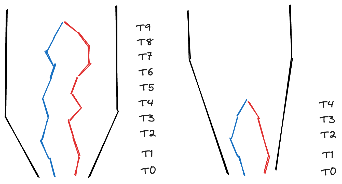
In addition, genetic diversity is impacted by demographic events and natural selection. Populations that have undergone a demographic expansion or contraction in the recent past will have distinct coalescent genealogies and therefore different genetic diversities. For instance, a population that has experienced a recent demographic expansion will have a TMRCA more recent than a population with the same population size that has remained stable through the same time period, illustrated below.
Distinguishing a small, constant-sized population from a large population that’s grown dramatically in the recent past is difficult with single-locus data typical of large-scale biodiversity studies. However, when paired with other data like traits and abundances, we can make more refined interpretations of the shape of genetic diversity across the community. For instance, the interpretation of a community with a few highly diverse species paired with many species with low genetic diversity may reflect a community with a few species that were not impacted by a historical environmental disturbance alongside many species that had their populations dramatically reduced, but have rapidly grown to larger modern population sizes.
Challenge
Draw one or more possible scenarios of a pair of coalescent genealogies drawn from a contracting population. The size of the modern and historical populations and the number of generations you “simulate” are up to you, but you should draw something similar to the figure above.
After completing this exercise, do you think a contracting population would result in more or less genetic diversity?
Contracting populations are funny! If a contraction was recent, the population may maintain the levels of genetic diversity it had before the contraction. However, if the contraction happened in the more distant past and was maintained, genetic diversity is reduced.
Hill numbers of genetic diversity across species
In the context of summarizing species abundances, Hill numbers are the effective number of species in a community, where each exponent (q-value) increasingly weights common species more heavily. The interpretation is similar when summarizing genetic diversity. Hill numbers are the effective number of species in a community, where each q-value increasingly weights species with higher genetic diversity more heavily. Rather than measuring an effective diversity of abundances, this is an effective diversity of genetic diversities.
Work with pop gen data
The three packages we’re working with are msa,
ape, and hillR. The first two are used to work
with sequencing data, while hillR is what we will use to
calculate Hill numbers. I’ll provide more explanation once we get to
using them.
R
library(msa)
library(ape)
library(hillR)
Sequences
FASTA
A FASTA file contains one or more DNA sequences, where the DNA sequence is preceded by a line with a carat (“>”) followed by an unique sequence ID:
>seq0010
GATCCCCAATTGGGG
This is perhaps the most common way to store sequence information as it is simple and has historical inertia. For more information, see the the NCBI page.
Alignment
Prior to analysis, sequence data must be aligned if they haven’t been already. A sequence alignment is necessary to identify regions of DNA that are similar or that vary. There are many pieces of software to perform alignments and all have their advantages and disadvantages, but we will choose a single program, Clustal Omega, which is fast and robust for short sequence alignments. While Clustal Omega can be run from the command line, we will use the R package msa to keep everything in the R environment.
First, a FASTA file containing the sequences needs to be read in
using the readDNAStringSet() function. For most of this
episode, we will be working with sequences from the Kauai island. At the
end, we will summarize the
R
seq_path <- "https://raw.githubusercontent.com/role-model/multidim-biodiv-data/main/episodes/data/kauai_seqs.fas"

seqs <- readDNAStringSet(seq_path)

seqs
OUTPUT
DNAStringSet object of length 130:
      width seq                                             names
  [1]   500 CGCGCACTCTACCACCCAGACT...TGACTCCTATCGTTAATTCGTG Proterhinus_punct...
  [2]   500 CGCGCACTCTACCACCCAGACT...TGACTCCTATCGTTAATTCGTG Proterhinus_punct...
  [3]   500 CGCGCACTCTACCACCCAGACT...TGACTCCTATCGTTAATTCGTG Proterhinus_punct...
  [4]   500 CGCGCACTCTACCACCCAGACT...TGACTCCTATCGTTAATTCGTG Proterhinus_punct...
  [5]   500 CGCGCACTCTACCACCCAGACT...TGACTCCTATCGTTAATTCGTG Proterhinus_punct...
  ...   ... ...
[126]   500 CGCGCACTCTACCACCCAGACT...TGACTCCTATCGTTAATTCGTG Campsicnemus_nigr...
[127]   500 CGCGCACTCTACCACCCAGACT...TGACTCCTATCGTTAATTCGTG Campsicnemus_nigr...
[128]   500 CGCGCACTCTACCACCCAGACT...TGACTCCTATCGTTAATTCGTG Campsicnemus_nigr...
[129]   500 CGCGCACTCTACCACCCAGACT...TGACTCCTATCGTTAATTCGTG Campsicnemus_nigr...
[130]   500 CGCGCACTCTACCACCCAGACT...TGACTCCTATCGTTAATTCGTG Campsicnemus_nigr...
To align the sequences using Clustal Omega, we use the
msa function and specify the method as
“ClustalOmega”. There are more arguments that you can use to fine-tune
the alignment, but these are not necessary for the vast majority of
scenarios.
R
alignment <- msa(seqs, method = "ClustalOmega")
OUTPUT
using GonnetR
alignment
OUTPUT
ClustalOmega 1.2.0

Call:
   msa(seqs, method = "ClustalOmega")

MsaDNAMultipleAlignment with 130 rows and 500 columns
      aln                                                  names
  [1] CGCGCACTCTACCACCCAGACTATC...CCGGACTCCTATCGATAATTCGTG Eudonia_lycopodiae-6
  [2] CGCGCACTCTACCACCCAGACTATC...CCCGACTCCTATCGTTAATTCGTG Eudonia_lycopodiae-1
  [3] CGCGCACTCTACCACCCAGACTATC...CCCGACTCCTATCGATAATTCGTG Eudonia_lycopodiae-4
  [4] CGCGCACTCTACCACCCAGACTATC...CCCGACTCCTATCGATAATTCGTG Eudonia_lycopodiae-3
  [5] CGCGCACTCTACCACCCAGACTATC...CCCGACTCCTATCGATAATTCGTG Eudonia_lycopodiae-8
  [6] CGCGCACTCTACCACCCAGACTATC...CCCGACTCCTATCGATAATTCGTG Eudonia_lycopodiae-2
  [7] CGCGCACTCTACCACCCAGACTATC...CCCGACTCCTATCGATAATTCGTG Eudonia_lycopodiae-5
  [8] CGCGCACTCTACCACCCAGACTATC...CCCGACTCCTATCGATAATTCGTG Eudonia_lycopodiae-9
  [9] CGCGCACTCTACCACCCAGACTATC...CCCGACTCCTATCGATAATTCGTG Eudonia_lycopodiae-0
  ... ...
[123] CGCGCACTCTACCACCCAGACTATC...CCTGACTCCTATCGTTAATTCGTG Nesodynerus_mimus-1
[124] CGCGCACTCTACCACCCAGACTATC...CCTGACTCCTATCGTTAATTCGTG Nesodynerus_mimus-5
[125] CGCGCACTCTACCACCCAGACTATC...CCTGACTCCTATCGTTAATTCGTG Nesodynerus_mimus-6
[126] CGCGCACTCTACCACCCAGACTATC...CCTGACTCCTATCGTTAATTCGTG Nesodynerus_mimus-7
[127] CGCGCACTCTACCACCCAGACTATC...CCTGACTCCTATCGTTAATTCGTG Nesodynerus_mimus-0
[128] CGCGCACTCTACCACCCAGACTATC...CCTGACTCCTATCGTTAATTCGTG Nesodynerus_mimus-8
[129] CGCGCACTCTACCACCCAGACTATC...CCTGACTCCTATCGTTAATTCGTG Nesodynerus_mimus-4
[130] CGCGCACTCTACCACCCAGACTATC...CCTGACTCCTATCGTTAATTCGTG Nesodynerus_mimus-9
  Con CGCGCACTCTACCACCCAGACTATC...CCTGACTCCTATCGTTAATTCGTG Consensus
If after you perform your alignment you find that one or more
individuals do not belong or are negatively impacting the alignment, you
have to manipulate your unaligned sequence data and then re-align the
sequences. For instance, say you didn’t want to include the individual
ind_name in the alignment. First, remove the individual
from the seqs object.
R
# remove individual
seqs_filt <- seqs[names(seqs) != "Eudonia_lycopodiae-6"]

seqs_filt
OUTPUT
DNAStringSet object of length 129:
      width seq                                             names
  [1]   500 CGCGCACTCTACCACCCAGACT...TGACTCCTATCGTTAATTCGTG Proterhinus_punct...
  [2]   500 CGCGCACTCTACCACCCAGACT...TGACTCCTATCGTTAATTCGTG Proterhinus_punct...
  [3]   500 CGCGCACTCTACCACCCAGACT...TGACTCCTATCGTTAATTCGTG Proterhinus_punct...
  [4]   500 CGCGCACTCTACCACCCAGACT...TGACTCCTATCGTTAATTCGTG Proterhinus_punct...
  [5]   500 CGCGCACTCTACCACCCAGACT...TGACTCCTATCGTTAATTCGTG Proterhinus_punct...
  ...   ... ...
[125]   500 CGCGCACTCTACCACCCAGACT...TGACTCCTATCGTTAATTCGTG Campsicnemus_nigr...
[126]   500 CGCGCACTCTACCACCCAGACT...TGACTCCTATCGTTAATTCGTG Campsicnemus_nigr...
[127]   500 CGCGCACTCTACCACCCAGACT...TGACTCCTATCGTTAATTCGTG Campsicnemus_nigr...
[128]   500 CGCGCACTCTACCACCCAGACT...TGACTCCTATCGTTAATTCGTG Campsicnemus_nigr...
[129]   500 CGCGCACTCTACCACCCAGACT...TGACTCCTATCGTTAATTCGTG Campsicnemus_nigr...
As a reminder, != means “does not equal”, so
names(seqs) != "Eudonia_lycopodiae-6" returns
TRUE when the sequence name does not match
“Eudonia_lycopodiae-6”.
Following the filtering, you need to realign the new set of sequences.
R
alignment <- msa(seqs_filt, method = "ClustalOmega")
OUTPUT
using GonnetR
alignment
OUTPUT
ClustalOmega 1.2.0

Call:
   msa(seqs_filt, method = "ClustalOmega")

MsaDNAMultipleAlignment with 129 rows and 500 columns
      aln                                                  names
  [1] CGCGCACTCTACCACCCAGACTATC...CCCGACTCCTATCGTTAATTCGTG Eudonia_lycopodiae-1
  [2] CGCGCACTCTACCACCCAGACTATC...CCCGACTCCTATCGATAATTCGTG Eudonia_lycopodiae-4
  [3] CGCGCACTCTACCACCCAGACTATC...CCCGACTCCTATCGATAATTCGTG Eudonia_lycopodiae-3
  [4] CGCGCACTCTACCACCCAGACTATC...CCCGACTCCTATCGATAATTCGTG Eudonia_lycopodiae-8
  [5] CGCGCACTCTACCACCCAGACTATC...CCCGACTCCTATCGATAATTCGTG Eudonia_lycopodiae-2
  [6] CGCGCACTCTACCACCCAGACTATC...CCCGACTCCTATCGATAATTCGTG Eudonia_lycopodiae-5
  [7] CGCGCACTCTACCACCCAGACTATC...CCCGACTCCTATCGATAATTCGTG Eudonia_lycopodiae-9
  [8] CGCGCACTCTACCACCCAGACTATC...CCCGACTCCTATCGATAATTCGTG Eudonia_lycopodiae-0
  [9] CGCGCACTCTACCACCCAGACTATC...CCCGACTCCTATCGATAATTCGTG Eudonia_lycopodiae-7
  ... ...
[122] CGCGCACTCTACCACCCAGACTATC...CCTGACTCCTATCGTTAATTCGTG Nesodynerus_mimus-1
[123] CGCGCACTCTACCACCCAGACTATC...CCTGACTCCTATCGTTAATTCGTG Nesodynerus_mimus-5
[124] CGCGCACTCTACCACCCAGACTATC...CCTGACTCCTATCGTTAATTCGTG Nesodynerus_mimus-6
[125] CGCGCACTCTACCACCCAGACTATC...CCTGACTCCTATCGTTAATTCGTG Nesodynerus_mimus-7
[126] CGCGCACTCTACCACCCAGACTATC...CCTGACTCCTATCGTTAATTCGTG Nesodynerus_mimus-0
[127] CGCGCACTCTACCACCCAGACTATC...CCTGACTCCTATCGTTAATTCGTG Nesodynerus_mimus-8
[128] CGCGCACTCTACCACCCAGACTATC...CCTGACTCCTATCGTTAATTCGTG Nesodynerus_mimus-4
[129] CGCGCACTCTACCACCCAGACTATC...CCTGACTCCTATCGTTAATTCGTG Nesodynerus_mimus-9
  Con CGCGCACTCTACCACCCAGACTATC...CCTGACTCCTATCGTTAATTCGTG Consensus
There are quite a few packages in R to work with sequence data, for
example seqinr,
phangorn,
and ape.
ape is the most versatile of these. But before we can use
ape, the alignment must be converted to the
ape::DNAbin format.
R
ape_align <- msaConvert(alignment, type = "ape::DNAbin")

ape_align
OUTPUT
129 DNA sequences in binary format stored in a matrix.

All sequences of same length: 500

Labels:
Eudonia_lycopodiae-1
Eudonia_lycopodiae-4
Eudonia_lycopodiae-3
Eudonia_lycopodiae-8
Eudonia_lycopodiae-2
Eudonia_lycopodiae-5
...

Base composition:
    a     c     g     t
0.260 0.245 0.234 0.261
(Total: 64.5 kb)
Although not necessary for this workshop (the sequence data is already aligned), it’s generally advisable to write your DNA alignment to a new file to use later or with other programs.
R
ape::write.FASTA(ape_align, "seqs_aligned.fas")
R
# you can also make a vector with the c() function and list each individual separately, but this requires a little less typing
hypo_inds <- paste0("Hyposmocoma_sagittata-", 0:9)

seqs_hypo <- seqs[names(seqs) %in% hypo_inds]

seqs_hypo
OUTPUT
DNAStringSet object of length 10:
     width seq                                              names
 [1]   500 CGCGCACTCTACCACCCAGACTA...TGACTCCTATCGTTAATTCGTG Hyposmocoma_sagit...
 [2]   500 CGCGCACTCTACCACCCAGACTA...TGACTCCTATCGTTAATTCGTG Hyposmocoma_sagit...
 [3]   500 CGCGCACTCTACCACCCAGACTA...TGACTCCTATCGTTAATTCGTG Hyposmocoma_sagit...
 [4]   500 CGCGCACTCTACCACCCAGACTA...TGACTCCTATCGTTAATTCGTG Hyposmocoma_sagit...
 [5]   500 CGCGCACTCTACCACCCAGACTA...TGACTCCTATCGTTAATTCGTG Hyposmocoma_sagit...
 [6]   500 CGCGCACTCTACCACCCAGACTA...TGACTCCTATCGTTAATTCGTG Hyposmocoma_sagit...
 [7]   500 CGCGCACTCTACCACCCAGACTA...TGACTCCTATCGTTAATTCGTG Hyposmocoma_sagit...
 [8]   500 CGCGCACTCTACCACCCAGACTA...TGACTCCTATCGTTAATTCGTG Hyposmocoma_sagit...
 [9]   500 CGCGCACTCTACCACCCAGACTA...TGACTCCTATCGTTAATTCGTG Hyposmocoma_sagit...
[10]   500 CGCGCACTCTACCACCCAGACTA...TGACTCCTATCGTTAATTCGTG Hyposmocoma_sagit...
ape
Check alignment
ape has a useful utility that allows you perform a
series of diagnostics on your alignment to make sure nothing is fishy.
The function can output multiple plots, but let’s just visualize the
alignment plot. If the colors seem jumbled in a region, this indicates
that an alignment error may have occurred and to inspect your sequences
for any problems.
In addition, the function outputs a series of helpful statistics to your console. Ideally, your alignment should have few gaps and a number of segregating sites that is reasonable for the number of sites in your alignment and the evolutionary divergence of the sequences included in the alignment, e.g., for an alignment with 970 sites of a single bird species, around 40 segregating sites is reasonable, but 200 segregating sites may indicate that something went wrong with your alignment or a species was misidentified. In addition, for diploid species a vast majority, if not all of the sites should contain one or two observed bases.
R
checkAlignment(ape_align, what = 1)
OUTPUT
Number of sequences: 129
Number of sites: 500

No gap in alignment.

Number of segregating sites (including gaps): 126
Number of sites with at least one substitution: 126
Number of sites with 1, 2, 3 or 4 observed bases:
  1   2   3   4
374 66 56 4 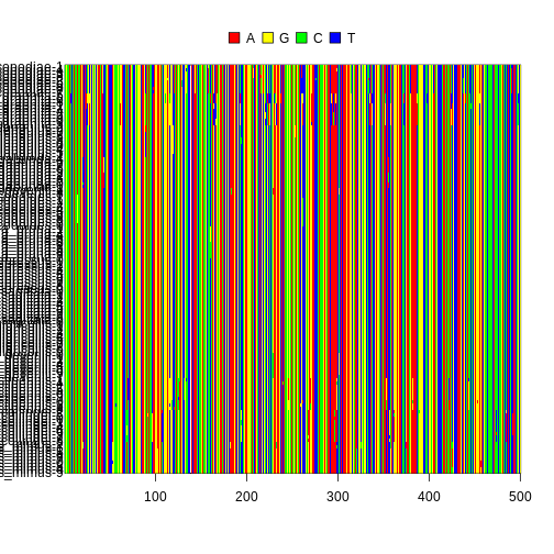
Calculate genetic diversity
To calculate genetic diversity for each species, it’s easiest to
split the alignment by species before calculating the average number of
pairwise nucleotide differences. Since we’re not concerned about
alignment quality, we can just split the alignment, rather than
splitting the original msa sequence object and
re-aligning.
First, you need to get the names of the species. Thankfully, the
genus and species is included in the sequences names, where the format
is “Genus_species-number”. To get the species names, you need to use the
gsub() function, which replaces all of the occurrences of a
particular string pattern in a string. In our case, we need to remove
the “-number” individual identifier at the end of the sequence name, so
we only have “Genus_species”. We will use a short regular expression, or
regex, which is a
sequence of characters that specifies a pattern that a string search
algorithm like gsub() will search for.
The pattern "-[0-9]" means “match any pattern in the
string that is a dash followed by any occurrence of a digit”. The hard
brackets [ ] specify a character set, where any occurrence
of the characters inside the brackets will be matched. In this case, we
specify zero through nine, so any digits that follow a dash will be
matched. The second argument contains the string to replace the pattern
with. We want to remove the pattern, so we supply an empty string to be
replaced.
Following the string removal, we only want unique instances of the
species names, so we use the unique() function to retain
unique species names.
R
sp_names <- gsub("-[0-9]", "", names(seqs))

sp_names <- unique(sp_names)

sp_names
OUTPUT
 [1] "Proterhinus_punctipennis" "Xyletobius_collingei"
 [3] "Metrothorax_deverilli"    "Nesodynerus_mimus"
 [5] "Scaptomyza_vagabunda"     "Lucilia_graphita"
 [7] "Eudonia_lycopodiae"       "Atelothrus_depressus"
 [9] "Mecyclothorax_longulus"   "Laupala_pruna"
[11] "Hylaeus_sphecodoides"     "Hyposmocoma_sagittata"
[13] "Campsicnemus_nigricollis"
Next, we are going to build an R function line-by-line to facilitate creating a list of species alignments. User-defined functions are very useful for when you want to complete a set of tasks repeatedly. Copy-pasting chunks of code and changing things slightly for each situation can lead to errors, headaches, and general pain. The worst bit of pain is when you need to change something in that chunk of code and you have to go back and change it for every instance you copy-pasted it before! When you have a function, you only need to change the code once. I’ll go through each line of code, then we’ll wrap up the code in a function.
First, we need to turn the ape alignment into a list
because the original DNAbin object doesn’t allow
subsetting.
R
align_list <- as.list(ape_align)
The grepl() function searches for a string pattern in
the text, then returns TRUE if it finds it and
FALSE if it doesn’t. We’ll use the resulting boolean
(TRUE/FALSE) vector to extract the species from the
alignment. Here is an example with Proterhinus punctipennis.
You’ll see the 100-110 slots are TRUE, indicating that
those are the locations in the alignment that contain P.
punctipennis sequences.
R
sp_boolean <- grepl("Proterhinus_punctipennis", names(align_list), fixed = TRUE)

sp_boolean
OUTPUT
  [1] FALSE FALSE FALSE FALSE FALSE FALSE FALSE FALSE FALSE FALSE FALSE FALSE
 [13] FALSE FALSE FALSE FALSE FALSE FALSE FALSE FALSE FALSE FALSE FALSE FALSE
 [25] FALSE FALSE FALSE FALSE FALSE FALSE FALSE FALSE FALSE FALSE FALSE FALSE
 [37] FALSE FALSE FALSE FALSE FALSE FALSE FALSE FALSE FALSE FALSE FALSE FALSE
 [49] FALSE FALSE FALSE FALSE FALSE FALSE FALSE FALSE FALSE FALSE FALSE FALSE
 [61] FALSE FALSE FALSE FALSE FALSE FALSE FALSE FALSE FALSE FALSE FALSE FALSE
 [73] FALSE FALSE FALSE FALSE FALSE FALSE FALSE FALSE FALSE FALSE FALSE FALSE
 [85] FALSE FALSE FALSE FALSE FALSE FALSE FALSE FALSE FALSE FALSE FALSE FALSE
 [97] FALSE FALSE FALSE  TRUE  TRUE  TRUE  TRUE  TRUE  TRUE  TRUE  TRUE  TRUE
[109]  TRUE FALSE FALSE FALSE FALSE FALSE FALSE FALSE FALSE FALSE FALSE FALSE
[121] FALSE FALSE FALSE FALSE FALSE FALSE FALSE FALSE FALSE
Following the conversion, we use bracket indexing to subset the
alignment by the sp_boolean boolean vector. Now we have an
alignment of only Proterhinus punctipennis sequences!
R
align_sp <- align_list[sp_boolean]

align_sp
OUTPUT
10 DNA sequences in binary format stored in a list.

All sequences of same length: 500

Labels:
Proterhinus_punctipennis-1
Proterhinus_punctipennis-4
Proterhinus_punctipennis-2
Proterhinus_punctipennis-5
Proterhinus_punctipennis-6
Proterhinus_punctipennis-9
...

Base composition:
    a     c     g     t
0.262 0.242 0.237 0.259
(Total: 5 kb)
Now, we need to wrap these bits of code into a function so we can create separate alignments for all species. The structure of a function looks like this.
R
do_something <- function(x, y) {

}
function() defines the do_something object
as a function, while x and y are the arguments
you are supplying to the function. The curly brackets { }
contain the code you want to run in the function.
For our function split_align, we need two arguments- the
species name we want to extract from the alignment (spname)
and the alignment itself (alignment). We then add our code
inside the curly brackets { }, replacing
"Proterhinus_punctipennis" with spname and
ape_align with alignment. At the end, we
specify that we want to return the align_sp object with the
return() function. Although not always necessary, using the
return() function is generally good practice for code
readability.
R
split_align <- function(spname, alignment) {
    # convert ape object to list
    align_list <- as.list(alignment)

    # get boolean vector for species
    sp_boolean <- grepl(spname, names(align_list), fixed = TRUE)

    # subset alignment for species
    align_sp <- align_list[sp_boolean]

    # return the alignment
    return(align_sp)
}
Now we can check that the function works by running it on Proterhinus punctipennis. It does! (or it should).
R
split_align(spname = "Proterhinus_punctipennis", alignment = ape_align)
OUTPUT
10 DNA sequences in binary format stored in a list.

All sequences of same length: 500

Labels:
Proterhinus_punctipennis-1
Proterhinus_punctipennis-4
Proterhinus_punctipennis-2
Proterhinus_punctipennis-5
Proterhinus_punctipennis-6
Proterhinus_punctipennis-9
...

Base composition:
    a     c     g     t
0.262 0.242 0.237 0.259
(Total: 5 kb)
If your code throws an error or the output isn’t what you expect, you
can place the browser() function at a particular line in
your code to enable you to run it line by line. This helps for
diagnosing where exactly something went wrong.
R
split_align <- function(spname, alignment) {
    browser()
    # convert ape object to list
    align_list <- as.list(alignment)

    # get boolean vector for species
    sp_boolean <- grepl(spname, names(align_list), fixed = TRUE)

    # subset alignment for species
    align_sp <- align_list[sp_boolean]

    # return the alignment
    return(align_sp)
}
Now to apply our function to the vector of species names! We’re using
the lapply() function to apply the split_seqs
function to every element in sp_names and return a list.
lapply() automatically populates the first argument in the
function with the vector or list you supply it, but you can supply
further arguments after entering your function. So, after adding
split_seqs, we specify
alignment = ape_align.
For good measure, we’ll also specify the names of the list elements as the species names, so they’re easy to access later.
R
align_split <- lapply(sp_names, split_align, alignment = ape_align)

names(align_split) <- sp_names

align_split
OUTPUT
$Proterhinus_punctipennis
10 DNA sequences in binary format stored in a list.

All sequences of same length: 500

Labels:
Proterhinus_punctipennis-1
Proterhinus_punctipennis-4
Proterhinus_punctipennis-2
Proterhinus_punctipennis-5
Proterhinus_punctipennis-6
Proterhinus_punctipennis-9
...

Base composition:
    a     c     g     t
0.262 0.242 0.237 0.259
(Total: 5 kb)

$Xyletobius_collingei
10 DNA sequences in binary format stored in a list.

All sequences of same length: 500

Labels:
Xyletobius_collingei-2
Xyletobius_collingei-5
Xyletobius_collingei-0
Xyletobius_collingei-1
Xyletobius_collingei-3
Xyletobius_collingei-4
...

Base composition:
    a     c     g     t
0.262 0.244 0.236 0.259
(Total: 5 kb)

$Metrothorax_deverilli
10 DNA sequences in binary format stored in a list.

All sequences of same length: 500

Labels:
Metrothorax_deverilli-2
Metrothorax_deverilli-8
Metrothorax_deverilli-0
Metrothorax_deverilli-1
Metrothorax_deverilli-3
Metrothorax_deverilli-4
...

Base composition:
    a     c     g     t
0.260 0.246 0.232 0.262
(Total: 5 kb)

$Nesodynerus_mimus
10 DNA sequences in binary format stored in a list.

All sequences of same length: 500

Labels:
Nesodynerus_mimus-2
Nesodynerus_mimus-3
Nesodynerus_mimus-1
Nesodynerus_mimus-5
Nesodynerus_mimus-6
Nesodynerus_mimus-7
...

Base composition:
    a     c     g     t
0.254 0.247 0.237 0.262
(Total: 5 kb)

$Scaptomyza_vagabunda
10 DNA sequences in binary format stored in a list.

All sequences of same length: 500

Labels:
Scaptomyza_vagabunda-4
Scaptomyza_vagabunda-6
Scaptomyza_vagabunda-7
Scaptomyza_vagabunda-8
Scaptomyza_vagabunda-9
Scaptomyza_vagabunda-2
...

Base composition:
    a     c     g     t
0.260 0.247 0.233 0.260
(Total: 5 kb)

$Lucilia_graphita
10 DNA sequences in binary format stored in a list.

All sequences of same length: 500

Labels:
Lucilia_graphita-5
Lucilia_graphita-6
Lucilia_graphita-8
Lucilia_graphita-1
Lucilia_graphita-7
Lucilia_graphita-4
...

Base composition:
    a     c     g     t
0.262 0.240 0.237 0.261
(Total: 5 kb)

$Eudonia_lycopodiae
9 DNA sequences in binary format stored in a list.

All sequences of same length: 500

Labels:
Eudonia_lycopodiae-1
Eudonia_lycopodiae-4
Eudonia_lycopodiae-3
Eudonia_lycopodiae-8
Eudonia_lycopodiae-2
Eudonia_lycopodiae-5
...

Base composition:
    a     c     g     t
0.258 0.248 0.231 0.262
(Total: 4.5 kb)

$Atelothrus_depressus
10 DNA sequences in binary format stored in a list.

All sequences of same length: 500

Labels:
Atelothrus_depressus-0
Atelothrus_depressus-1
Atelothrus_depressus-2
Atelothrus_depressus-3
Atelothrus_depressus-4
Atelothrus_depressus-5
...

Base composition:
    a     c     g     t
0.260 0.246 0.232 0.262
(Total: 5 kb)

$Mecyclothorax_longulus
10 DNA sequences in binary format stored in a list.

All sequences of same length: 500

Labels:
Mecyclothorax_longulus-2
Mecyclothorax_longulus-9
Mecyclothorax_longulus-7
Mecyclothorax_longulus-8
Mecyclothorax_longulus-3
Mecyclothorax_longulus-6
...

Base composition:
    a     c     g     t
0.260 0.244 0.235 0.261
(Total: 5 kb)

$Laupala_pruna
10 DNA sequences in binary format stored in a list.

All sequences of same length: 500

Labels:
Laupala_pruna-1
Laupala_pruna-2
Laupala_pruna-4
Laupala_pruna-8
Laupala_pruna-9
Laupala_pruna-0
...

Base composition:
    a     c     g     t
0.260 0.247 0.233 0.260
(Total: 5 kb)

$Hylaeus_sphecodoides
10 DNA sequences in binary format stored in a list.

All sequences of same length: 500

Labels:
Hylaeus_sphecodoides-7
Hylaeus_sphecodoides-1
Hylaeus_sphecodoides-2
Hylaeus_sphecodoides-3
Hylaeus_sphecodoides-4
Hylaeus_sphecodoides-5
...

Base composition:
    a     c     g     t
0.258 0.248 0.234 0.260
(Total: 5 kb)

$Hyposmocoma_sagittata
10 DNA sequences in binary format stored in a list.

All sequences of same length: 500

Labels:
Hyposmocoma_sagittata-0
Hyposmocoma_sagittata-1
Hyposmocoma_sagittata-2
Hyposmocoma_sagittata-3
Hyposmocoma_sagittata-4
Hyposmocoma_sagittata-5
...

Base composition:
    a     c     g     t
0.260 0.246 0.232 0.262
(Total: 5 kb)

$Campsicnemus_nigricollis
10 DNA sequences in binary format stored in a list.

All sequences of same length: 500

Labels:
Campsicnemus_nigricollis-0
Campsicnemus_nigricollis-1
Campsicnemus_nigricollis-2
Campsicnemus_nigricollis-3
Campsicnemus_nigricollis-4
Campsicnemus_nigricollis-5
...

Base composition:
    a     c     g     t
0.260 0.246 0.232 0.262
(Total: 5 kb)
Now we’re going to calculate the average number of pairwise genetic
differences among these sequences. ape has the
dist.dna() function to calculate various genetic distance
metrics for an alignment.
You use the argument model = "raw" to specify that you
want to use the average number of pairwise differences as your metric.
When calculating the number of pairwise genetic differences, you have to
choose whether you want missing data to be deleted across the entire
alignment (pairwise.deletion = FALSE) or only between the
two sequences being compared (pairwise.deletion = TRUE).
Since we want to take advantage of as much data as possible when
computing 𝜋, we’ll set pairwise.deletion = TRUE.
We’ll do this for a single species, then you’ll get a chance to write your own function to do it across species!
R
fas_gendist <- dist.dna(align_split$Proterhinus_punctipennis, model = "raw", pairwise.deletion = TRUE)

fas_gendist
OUTPUT
                           Proterhinus_punctipennis-1
Proterhinus_punctipennis-4                      0.010
Proterhinus_punctipennis-2                      0.006
Proterhinus_punctipennis-5                      0.006
Proterhinus_punctipennis-6                      0.006
Proterhinus_punctipennis-9                      0.006
Proterhinus_punctipennis-7                      0.008
Proterhinus_punctipennis-0                      0.026
Proterhinus_punctipennis-3                      0.028
Proterhinus_punctipennis-8                      0.024
                           Proterhinus_punctipennis-4
Proterhinus_punctipennis-4
Proterhinus_punctipennis-2                      0.004
Proterhinus_punctipennis-5                      0.004
Proterhinus_punctipennis-6                      0.004
Proterhinus_punctipennis-9                      0.004
Proterhinus_punctipennis-7                      0.006
Proterhinus_punctipennis-0                      0.024
Proterhinus_punctipennis-3                      0.026
Proterhinus_punctipennis-8                      0.022
                           Proterhinus_punctipennis-2
Proterhinus_punctipennis-4
Proterhinus_punctipennis-2
Proterhinus_punctipennis-5                      0.000
Proterhinus_punctipennis-6                      0.000
Proterhinus_punctipennis-9                      0.000
Proterhinus_punctipennis-7                      0.002
Proterhinus_punctipennis-0                      0.020
Proterhinus_punctipennis-3                      0.022
Proterhinus_punctipennis-8                      0.018
                           Proterhinus_punctipennis-5
Proterhinus_punctipennis-4
Proterhinus_punctipennis-2
Proterhinus_punctipennis-5
Proterhinus_punctipennis-6                      0.000
Proterhinus_punctipennis-9                      0.000
Proterhinus_punctipennis-7                      0.002
Proterhinus_punctipennis-0                      0.020
Proterhinus_punctipennis-3                      0.022
Proterhinus_punctipennis-8                      0.018
                           Proterhinus_punctipennis-6
Proterhinus_punctipennis-4
Proterhinus_punctipennis-2
Proterhinus_punctipennis-5
Proterhinus_punctipennis-6
Proterhinus_punctipennis-9                      0.000
Proterhinus_punctipennis-7                      0.002
Proterhinus_punctipennis-0                      0.020
Proterhinus_punctipennis-3                      0.022
Proterhinus_punctipennis-8                      0.018
                           Proterhinus_punctipennis-9
Proterhinus_punctipennis-4
Proterhinus_punctipennis-2
Proterhinus_punctipennis-5
Proterhinus_punctipennis-6
Proterhinus_punctipennis-9
Proterhinus_punctipennis-7                      0.002
Proterhinus_punctipennis-0                      0.020
Proterhinus_punctipennis-3                      0.022
Proterhinus_punctipennis-8                      0.018
                           Proterhinus_punctipennis-7
Proterhinus_punctipennis-4
Proterhinus_punctipennis-2
Proterhinus_punctipennis-5
Proterhinus_punctipennis-6
Proterhinus_punctipennis-9
Proterhinus_punctipennis-7
Proterhinus_punctipennis-0                      0.022
Proterhinus_punctipennis-3                      0.024
Proterhinus_punctipennis-8                      0.020
                           Proterhinus_punctipennis-0
Proterhinus_punctipennis-4
Proterhinus_punctipennis-2
Proterhinus_punctipennis-5
Proterhinus_punctipennis-6
Proterhinus_punctipennis-9
Proterhinus_punctipennis-7
Proterhinus_punctipennis-0
Proterhinus_punctipennis-3                      0.014
Proterhinus_punctipennis-8                      0.010
                           Proterhinus_punctipennis-3
Proterhinus_punctipennis-4
Proterhinus_punctipennis-2
Proterhinus_punctipennis-5
Proterhinus_punctipennis-6
Proterhinus_punctipennis-9
Proterhinus_punctipennis-7
Proterhinus_punctipennis-0
Proterhinus_punctipennis-3
Proterhinus_punctipennis-8                      0.008
The function returns a distance matrix containing the pairwise
differences among all sequences in the data set. To take a quick peak at
their distribution, we can use the hist() function on the
distance matrix.
R
hist(fas_gendist)
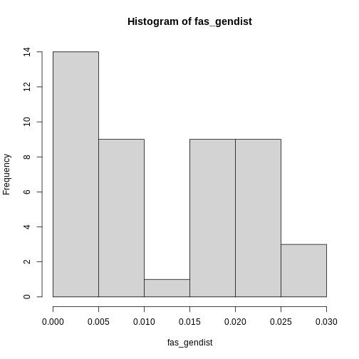
Since we want the average of these differences, we need to take their
average. However, you may have noticed the distribution of genetic
distances is non-normal, with mostly low genetic diversities. This is
the case with most genetic data sets. So, instead of taking the mean,
the median() will provide a better estimate of the center
of the distribution. The average number of pairwise genetic differences,
aka 𝜋, aka genetic diversity of Proterhinus punctipennis is
0.01!
R
fas_gendiv <- median(fas_gendist)

fas_gendiv
OUTPUT
[1] 0.01R
calc_pi <- function(alignment) {
    # get genetic distances
    dists <- dist.dna(alignment, model = "raw", pairwise.deletion = TRUE)
    # get average
    pi <- median(dists)

    return(pi)
}
I haven’t introduced it yet, but sapply() is similar to
lapply(), except it returns a vector instead of a list. It
saves an extra step when you know your function is returning single
values of the same type.
R
# solution 1. This returns a vector
pi_across_sp <- sapply(align_split, calc_pi)

# solution 2
pi_across_sp <- lapply(align_split, calc_pi)
## convert to a vector
pi_across_sp <- unlist(pi_across_sp)
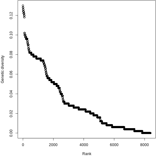
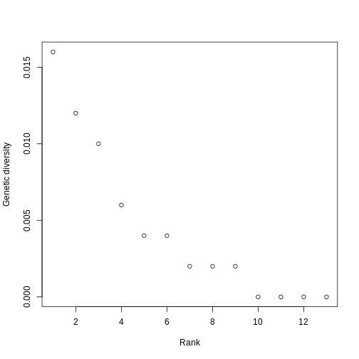
Let’s plot the ranked genetic diversities of Kauai! We’ll use plotting techniques similar to what you’ve used in the Abundance and Traits episodes.
R
plot(sort(pi_across_sp, decreasing = TRUE), xlab = "Rank", ylab = "Genetic diversity")
Hill numbers
Now, let’s calculate the first five Hill numbers (q = 1-5) of this
distribution. For this, we will use the hillR package.
hillR does not have a function specifically for calculating
Hill numbers from genetic diversities, but the function you have used
for calculating Hill numbers from abundances, hill_taxa
will work the same.
To turn your vector of genetic diversities into a site by species
matrix, you just need to transpose pi_across_sp with the
t() function. This turns pi_across_sp into a
matrix with a column for each species and a row for each site, which in
this case is 1.
R
pi_t <- t(pi_across_sp)
pi_t
OUTPUT
     Proterhinus_punctipennis Xyletobius_collingei Metrothorax_deverilli
[1,]                     0.01                0.006                 0.002
     Nesodynerus_mimus Scaptomyza_vagabunda Lucilia_graphita Eudonia_lycopodiae
[1,]             0.004                0.004            0.016              0.012
     Atelothrus_depressus Mecyclothorax_longulus Laupala_pruna
[1,]                    0                  0.002         0.002
     Hylaeus_sphecodoides Hyposmocoma_sagittata Campsicnemus_nigricollis
[1,]                    0                     0                        0
Finally, you can feed this matrix into hill_taxa() for
each q value we’re interested in. To make this efficient, let’s use
sapply()!
R
hill_pi <- sapply(1:5, hill_taxa, comm = pi_t)
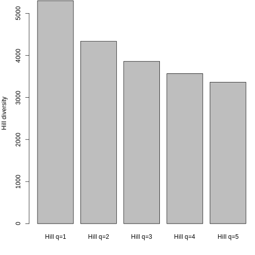
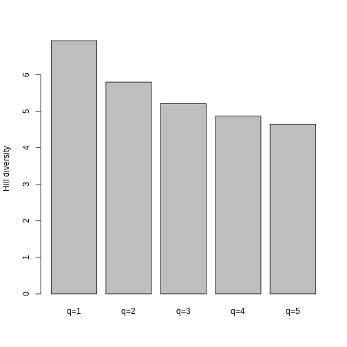
A quick barplot shows what we expect- Hill decreases with increasing q because it is increasingly weighted by low genetic diversities.
R
barplot(hill_pi, names.arg = c("q=1", "q=2", "q=3", "q=4", "q=5"), ylab = "Hill diversity")
Comparison across islands
Challenge
Lets go through the whole workflow for the Big Island and Maui! Go from the raw sequences to per-species Hill numbers of genetic diversity for both islands. After the challenge we’ll plot genetic diversities and Hill numbers across all three islands and compare!
R
# big island fasta
seqs_bi <- readDNAStringSet("https://raw.githubusercontent.com/role-model/multidim-biodiv-data/main/episodes/data/big_island_seqs.fas")
# maui fasta
seqs_maui <- readDNAStringSet("https://raw.githubusercontent.com/role-model/multidim-biodiv-data/main/episodes/data/maui_seqs.fas")
If you had more islands or localities, you could make a mega-function to get the genetic diversities and/or Hill numbers of each of the localities, rather than copy-pasting this code repeatedly. Functions are very useful!
R
# big island
## align sequences
align_bi <- msa(seqs_bi, method = "ClustalOmega")
OUTPUT
using GonnetR
## convert to DNAbin
ape_align_bi <- msaConvert(align_bi, type = "ape::DNAbin")
## unique names to create alignment list
sp_bi <- unique(gsub("-[0-9]", "", names(seqs_bi)))
## split alignment into list of each species
align_list_bi <- lapply(sp_bi, split_align, alignment = ape_align_bi)
## add names to alignment list
names(align_list_bi) <- sp_bi
## get genetic diversities
pi_bi <- sapply(align_list_bi, calc_pi)
## get Hill numbers 1:5
hill_bi <- sapply(1:5, hill_taxa, comm = t(pi_bi))

# maui
## align sequences
align_maui <- msa(seqs_maui, method = "ClustalOmega")
OUTPUT
using GonnetR
## convert to DNAbin
ape_align_maui <- msaConvert(align_maui, type = "ape::DNAbin")
## unique names to create alignment list
sp_maui <- unique(gsub("-[0-9]", "", names(seqs_maui)))
## split alignment into list of each species
align_list_maui <- lapply(sp_maui, split_align, alignment = ape_align_maui)
## add names to alignment list
names(align_list_maui) <- sp_maui
## get genetic diversities
pi_maui <- sapply(align_list_maui, calc_pi)
## get Hill numbers 1:5
hill_maui <- sapply(1:5, hill_taxa, comm = t(pi_maui))
Now, let’s plot the ranked genetic diversities of each island on the
same plot to compare their shapes. A line plot shows the general shape
of the trend a little clearer, so we’ll set type = "l". We
will use Maui as the base plot, since it has the most species. Then,
we’ll add the other two islands to the plot using the
lines() function.
R
plot(sort(pi_maui, TRUE), type = "l", xlab = "Rank", ylab = "Genetic diversity")
lines(sort(pi_bi, TRUE), col = "red")
lines(sort(pi_across_sp, TRUE), col = "blue")
legend("topright", c("Maui", "Big Island", "Kauai"), fill = c("black", "red", "blue"))
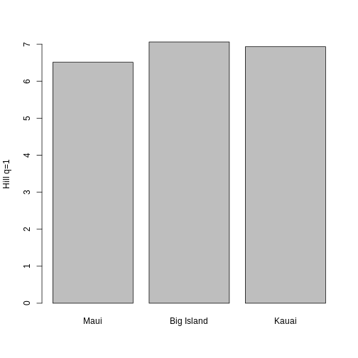
Now, let’s compare Hill q=1 across the three islands. An interesting pattern that we see is that even though Maui has more species, the Hill diversities of the Big Island and Kauai are larger! What is a potential interpretation of these data, especially in light of the abundance and traits data?
R
barplot(c(hill_maui[1], hill_bi[1], hill_pi[1]), names.arg = c("Maui", "Big Island", "Kauai"), ylab = "Hill q=1")
ASVs and Metabarcoding
Metabarcoding is rapidly growing DNA sequencing method used for biodiversity assessment. It involves sequencing a short, variable region of DNA sequence across a sample that may contain many taxa. This can be used to rapidly assess the diversity of a particular sampling site with low sampling effort. Some common applications include microbiome diversity assessments, environmental DNA, and community DNA. In many applications where a data base of species identities for sequence variants is not available or desired, the diversity of sequences is inferred, rather than the diversity of species. Additionally, while there are caveats, the relative abundance of sequences can be considered analogous to the relative abundance of species across a community.
The basic unit of diversity used in most studies is the amplicon sequence variant (ASV). An ASV is any one of the sequences inferred from a high-throughput sequencing experiment. These sequences are free from errors and may diverge by as little as a single base pair from each other. They are considered a substitute for operational taxonomic units (OTUs) for evaluating ecological diversity given their higher resolution, reproducibility, and no need for a reference database.
Sequence table
The basic unit of analysis used for metabarcoding studies is the sequence table. It is a matrix with named rows corresponding to the samples and named columns corresponding to the ASVs. Each cell contains the count of each variant in each sample. Here’s an example with 5 samples and 4 sequence variants:
| asv_1 | asv_2 | asv_3 | asv_4 | |
|---|---|---|---|---|
| sample_1 | 0 | 276 | 200 | 10 |
| sample_2 | 10 | 1009 | 0 | 0 |
| sample_3 | 0 | 0 | 234 | 15 |
| sample_4 | 129 | 1992 | 0 | 485 |
| sample_5 | 1001 | 10 | 1847 | 178 |
sample_1 may correspond to a soil sample collected in a forest, while the variants represent different ASVs, which could look like this:
asv_1: GTTCA
asv_2: GTACA
asv_3: GATCA
asv_4: CTTCA
This looks similiar to a site by species matrix, where the rows are a sampling locality, the columns are the species, and the cell values are the abundance of a species at a particular site.
We’ll briefly go over how the data makes its way from raw sequencing data to the sequence table.
DADA2
DADA2 is one of the most powerful and commonly used software packages for processing raw ASV sequencing data to turn it into a table of ASVs for each sample. This workshop assumes you are using the output from this workflow for further analysis, but for clarity the steps to the workflow include:
- read quality assessment
- filtering and trimming FASTQ files
- learning sequencing error rates, so the algorithm can correct for them
- infer the sequence variants
- merging paired reads (if sequencing was done with forward and reverse read pairs)
- constructing a sequence table
The raw reads are typically in the FASTQ format, which is similar to FASTA, but with some added metadata about the sequences. For more in-depth discussion about FASTQ format, you can scroll to the Extra section!
There are more available to further assess the quality of the data and map the data to taxonomic databases, but the core output of DADA2 and similar software pipelines is the sequence table.
Comparison with sequence alignment workflow
You can analyze ASV data in two ways. You can use the ASV sequencing
table directly and use abundances of each ASV as input into the
hill_taxa() function, considering each ASV as its own
“species”. This has the advantage of using the ASV’s quality as a
minimal reproducible taxonomic unit.
Alternatively, if you have a taxonomic reference database, you can map each ASV to its species identity, convert the table into a FASTA alignment, then calculate metrics like the average number of pairwise nucleotide differences per species. This has the advantage of being able to directly compare genetic diversity metrics with other dimensions of biodiversity like traits and abundances among species. However, the sequence lengths used for ASVs are typically very short and may not capture sufficient variation to characterize species diversity.
Extra
FASTQ
The FASTQ file format is similar to the FASTA format introduced earlier, but includes additional data about the contained sequences. This enables more flexible data manipulation and filtering capabilities, and is popular with high-throughput sequencing technologies. When working with ASVs, this is the most common file format you will encounter.
A FASTA formatted sequence may look like this,
>seq1
GATTTGGGGTTCAAAGCAGTATCGATCAAATAGTAAATCCATTTGTTCAACTCACAGTTT
while a FASTQ version of the same sequence may look like this:
@seq1
GATTTGGGGTTCAAAGCAGTATCGATCAAATAGTAAATCCATTTGTTCAACTCACAGTTT
+
!''*((((***+))%%%++)(%%%%).1***-+*''))**55CCF>>>>>>CCCCCCC65
If your eyes glaze over at the seemingly random numbers below the sequence, don’t fret! They mean something, but usually your machine does the interpreting for you. A FASTQ file is formatted as follows:
An ‘@’ symbol followed by a sequence identifier and an optional description
The raw sequence letters
A ‘+’ character that is optionally followed by the sequence identifier and more description
Quality encodings for the raw sequence letters in field 2. There must be the same number of encoding symbols as there are sequence letters.
The symbols are bytes representing quality, ranging from 0x21 (lowest quality; ‘!’ in ASCII) to 0x7e (highest quality; ‘~’ in ASCII). Here, they’re arranged in order of quality from lowest on the left to highest on the right:
!"#$%&'()*+,-./0123456789:;<=>?@ABCDEFGHIJKLMNOPQRSTUVWXYZ[\]^_`abcdefghijklmnopqrstuvwxyz{|}~Fortunately, whatever bioinformatic program you use will generally do the interpreting for you.
Different sequencing technologies (e.g. Illumina) have standardized description strings which contain more information about the sequences and can be useful when filtering sequences or performing QC. For examples, see the Wikipedia page.